
A CLEARER WAY TO TEACH SCIENCE
Big ideas.
Beautifully visible.
Science visuals for the moment a concept needs to click. Find the right level of detail for your next lesson, slide or worksheet.
Explore the library ↓Explore Biology, Chemistry and Physics. Find your level of detail.

THE VISUAL LIBRARY
Find your next explanation.
150 concepts + 119 apparatus setups · 1,107 visuals
Explore 150 concepts, each in five levels of detail.
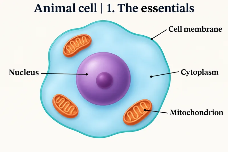 BIOLOGY · 5 VISUALSAnimal cellStart with the essentials. Reveal more detail when your class is ready.
The essentials
A simple, labelled overview for introducing the main cell structures.
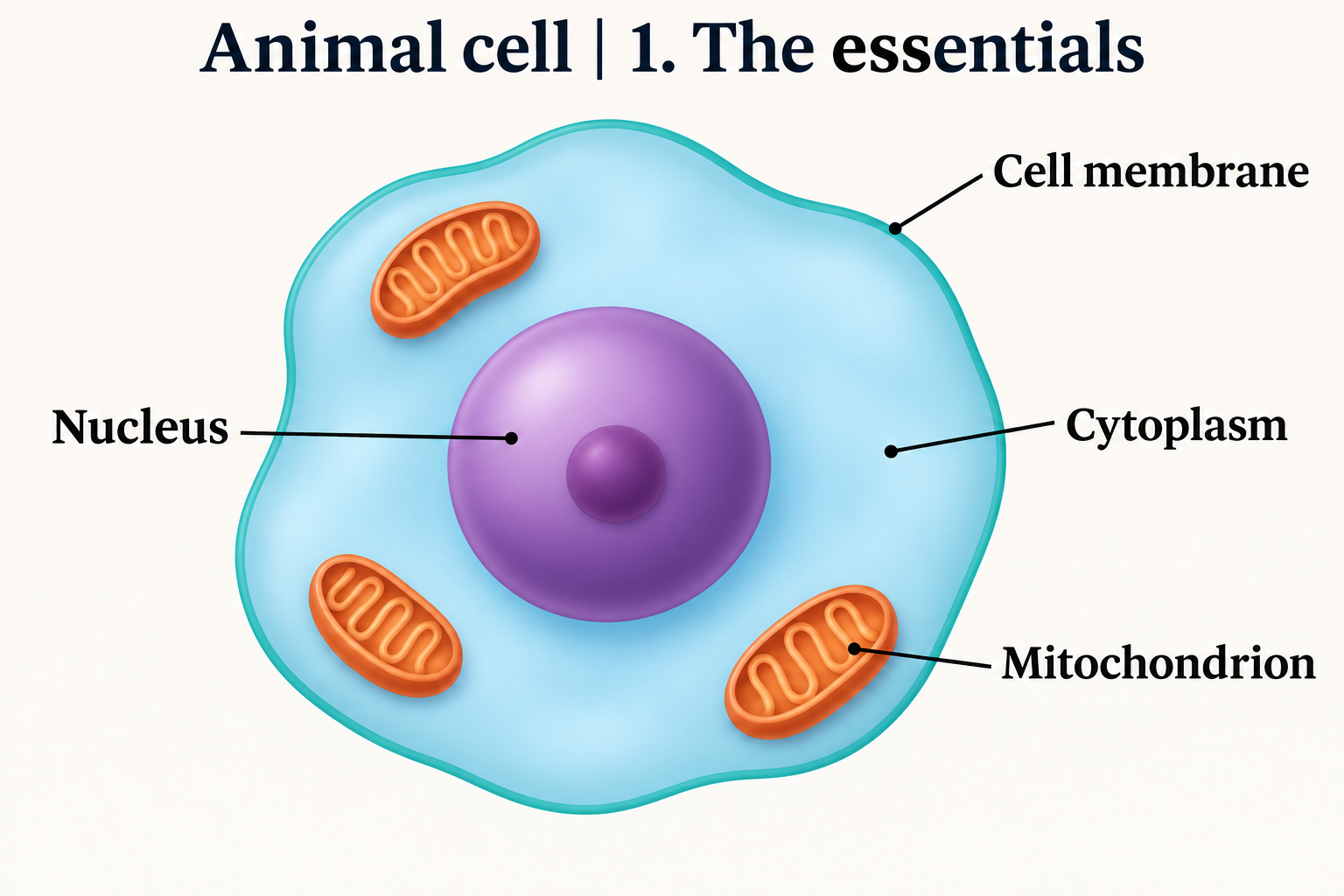

Inside the cell
A labelled view of the organelles and the spaces around them.


Cellular architecture
A richer cutaway that brings the internal structures into focus.


Membranes and organelles
A detailed view for looking more closely at the cell’s organisation.


The cellular world
An intricate illustration with layers of internal cellular detail.

 BIOLOGY · 5 VISUALSPlant cellExplore plant-cell structures, a mesophyll cell and contrasting turgor states.
Plant cell essentials
A labelled introduction to the cell wall, membrane, nucleus, chloroplasts and central vacuole.


Cellular structures
Look more closely at the organelles, plasma membrane and tonoplast.


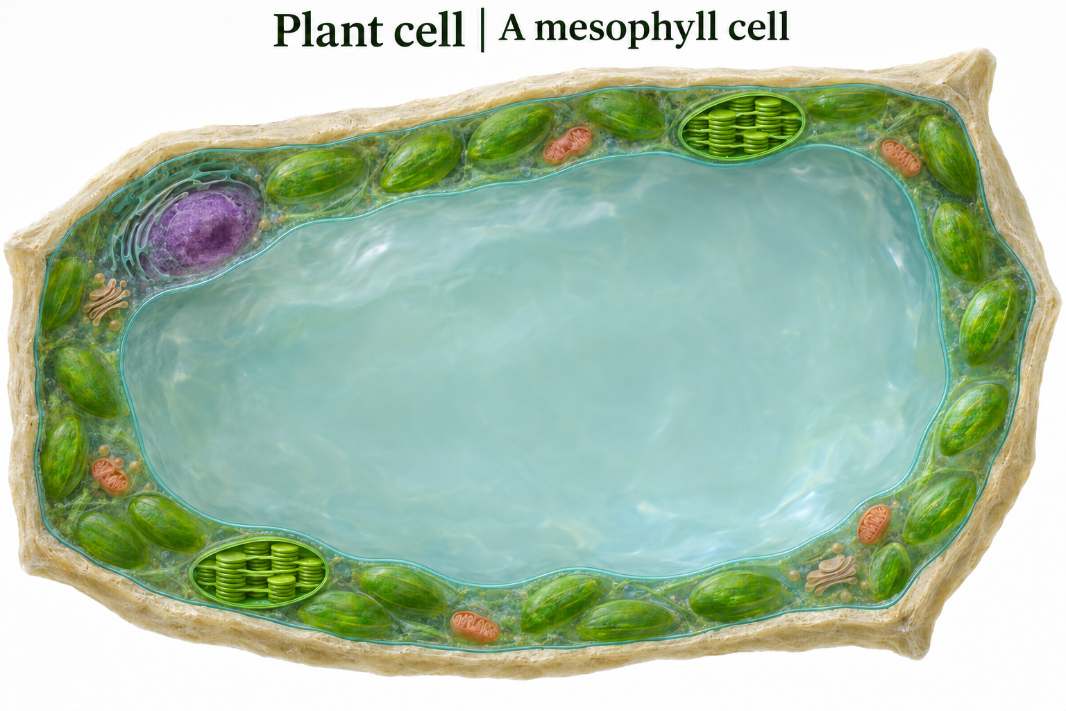
A mesophyll cell
An unlabelled cutaway for exploring a leaf cell and its chloroplasts.
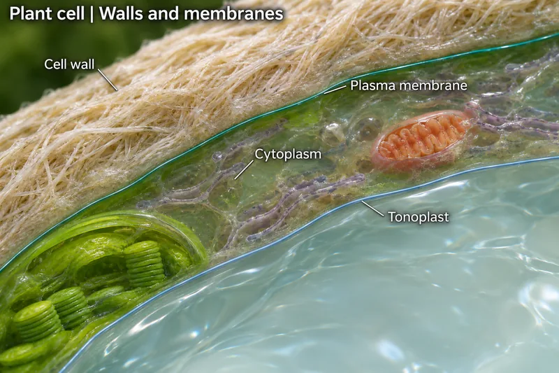
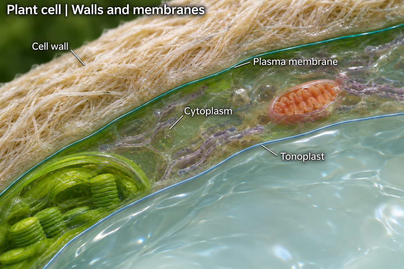
Walls and membranes
A detailed cutaway for discussing the cell wall and internal organisation.

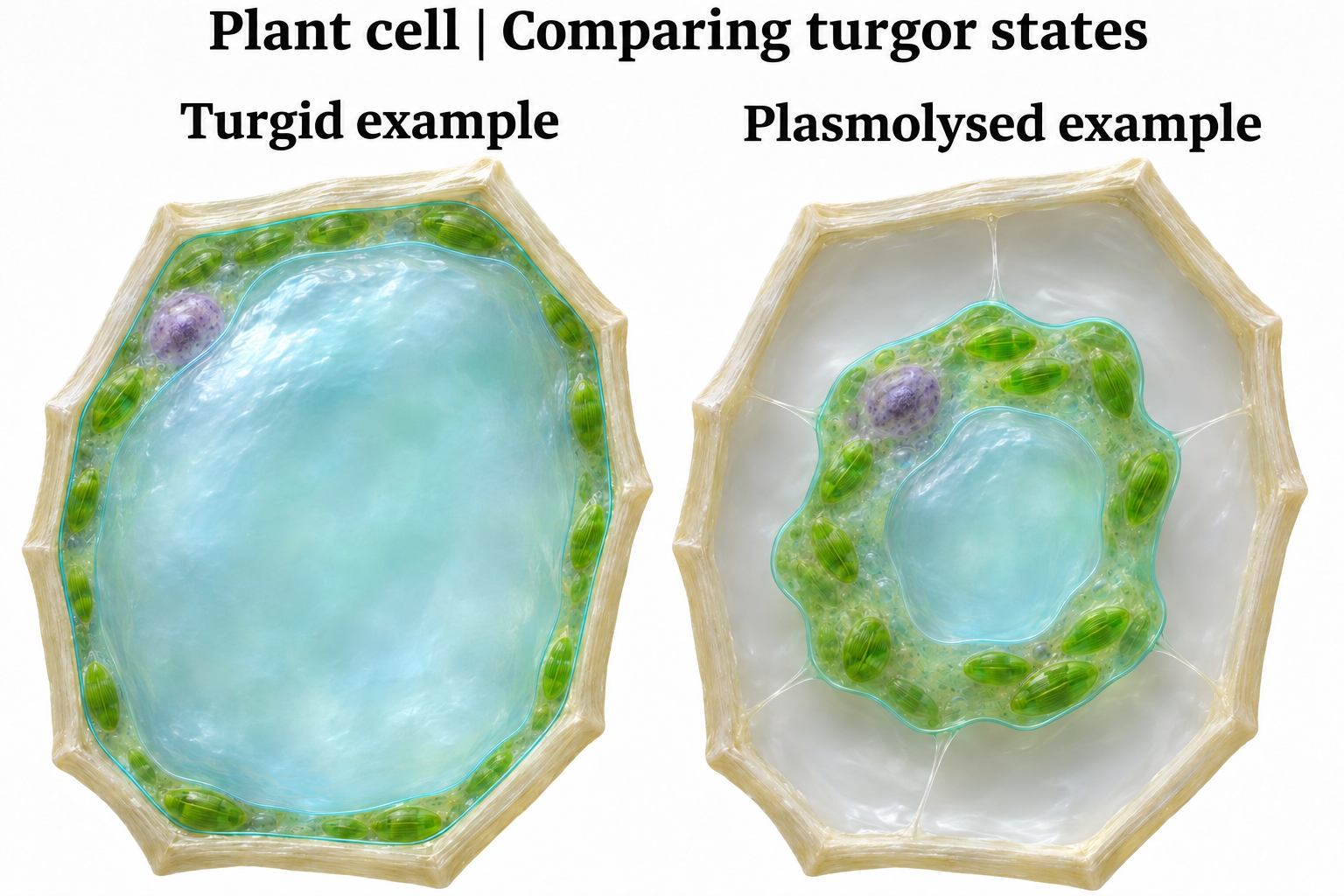
Comparing turgor states
Compare a turgid example with a plasmolysed example when explaining water movement.
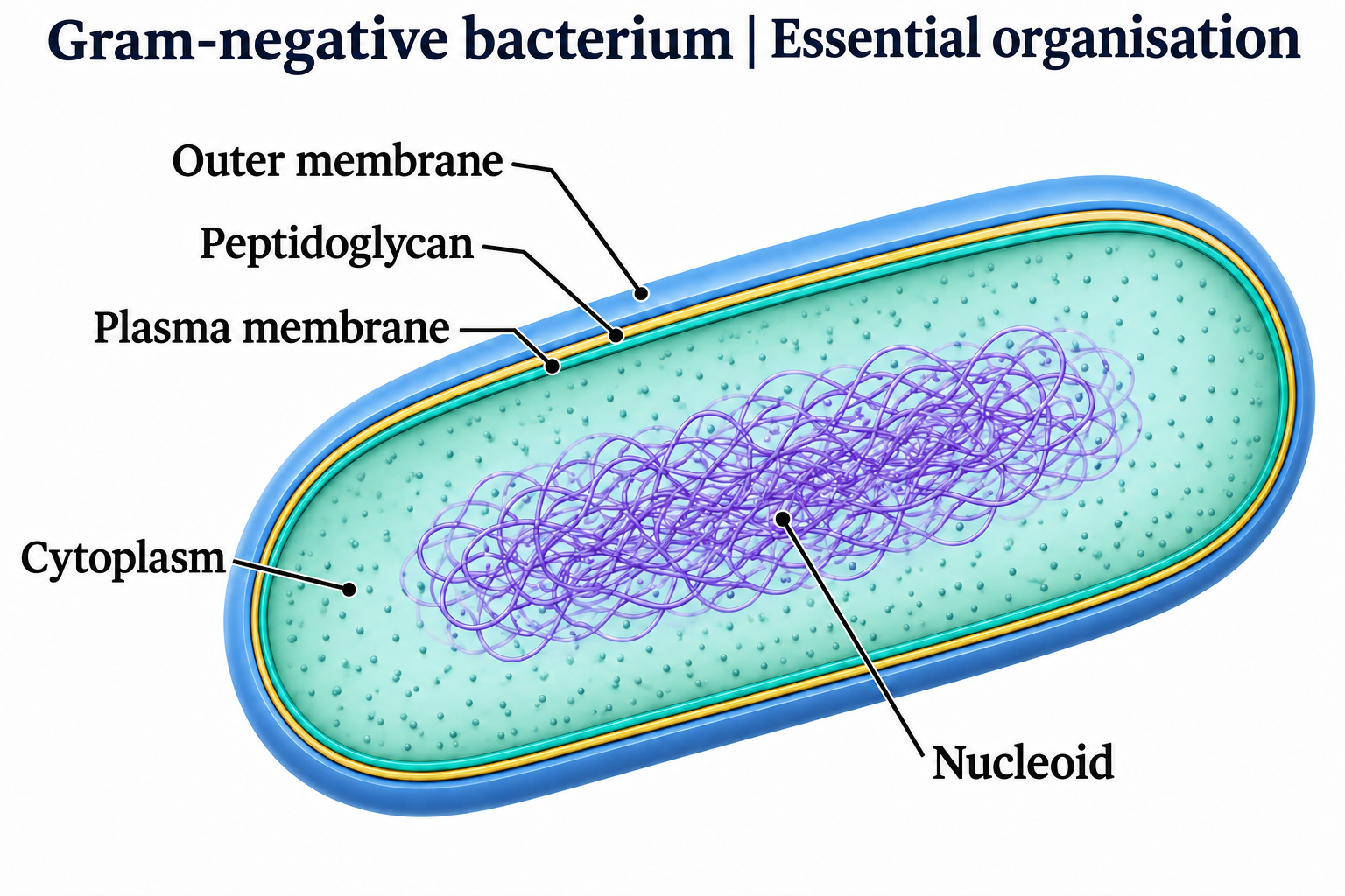
 BIOLOGY · 5 VISUALSBacterial cellExplore bacterial examples, envelope types and comparisons with human cells.
Bacterial cell essentials
A labelled introduction to a bacterial-cell example and its main structures.

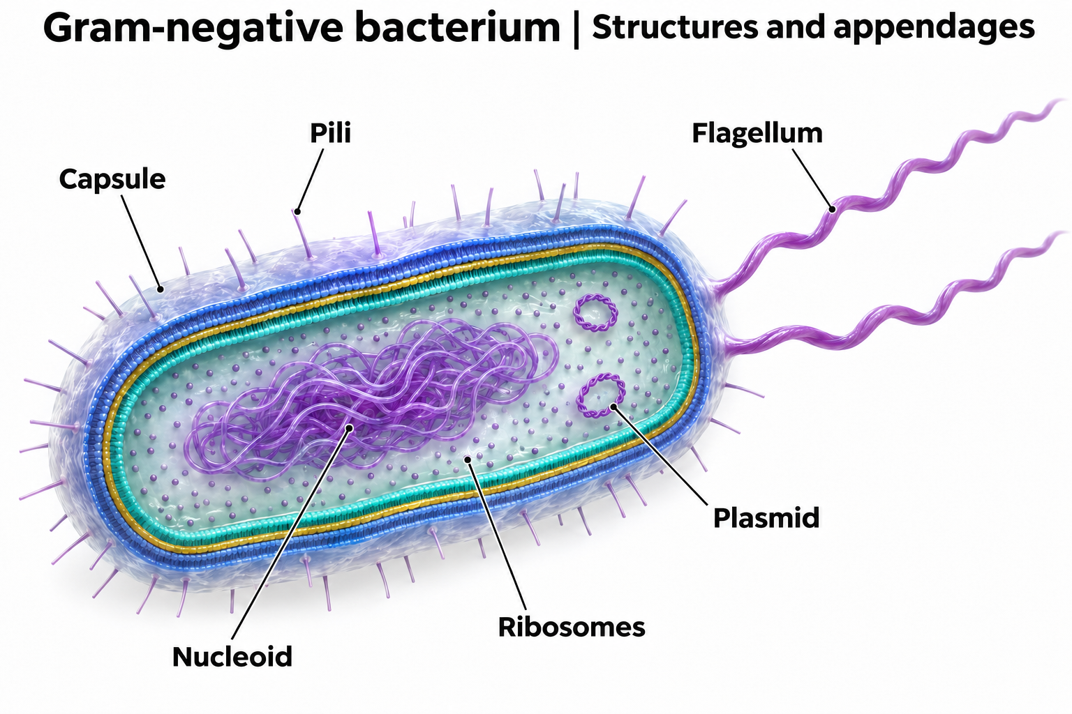
Bacterial structures
Explore structures shown in this bacterial example, including the genetic material and cell envelope.

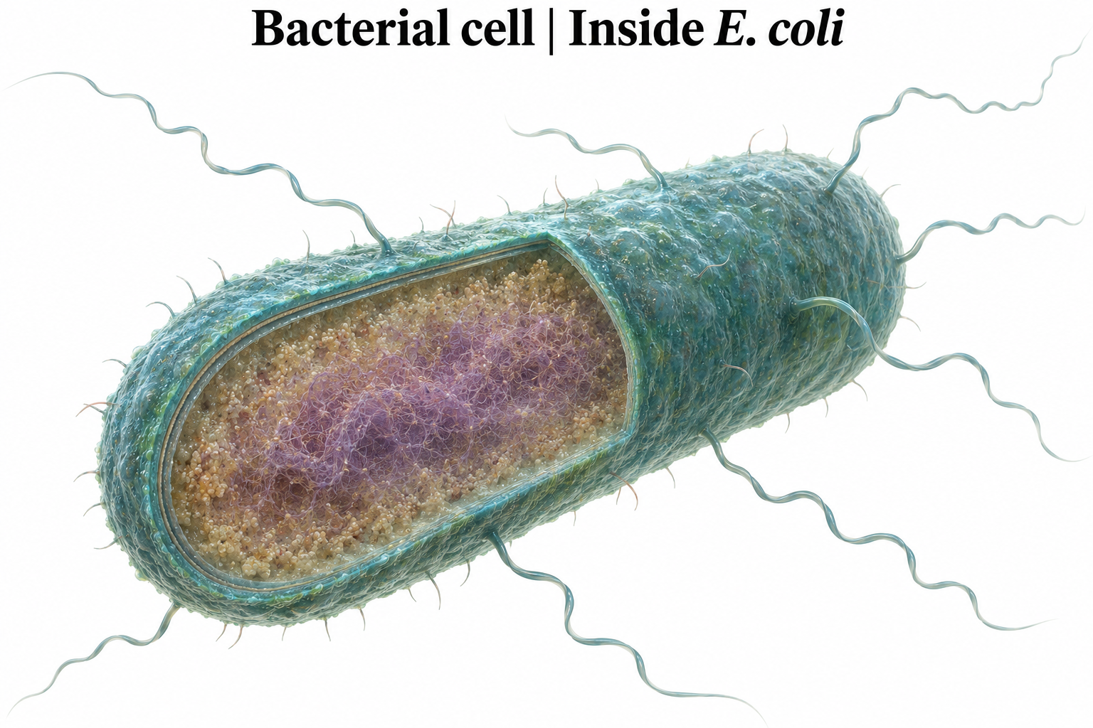
An E. coli example
A detailed cutaway for exploring the organisation of an E. coli cell.

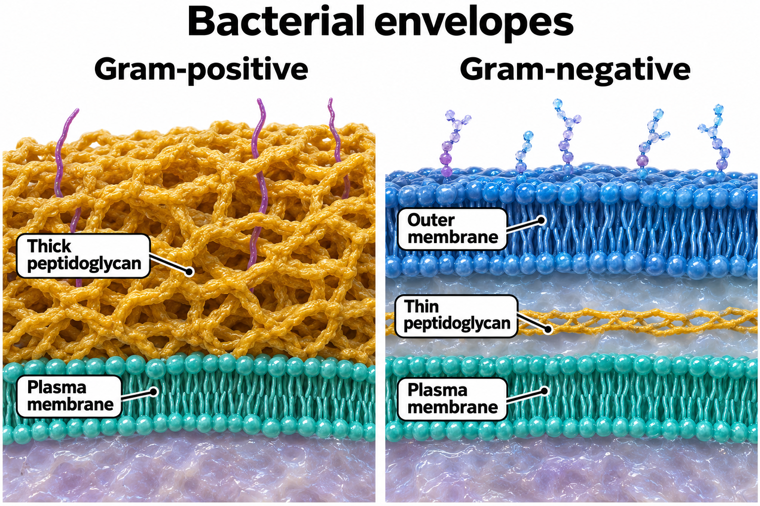
Comparing cell envelopes
Compare the cell-envelope layers shown in Gram-positive and Gram-negative bacterial examples.

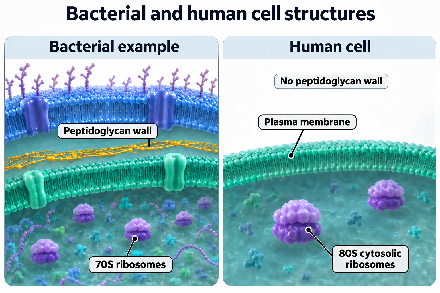
Bacterial and human cell structures
Compare selected envelope and ribosome features in a bacterial example and a human cell.
 BIOLOGY · 5 VISUALSCell membraneExplore the lipid bilayer, fluid mosaic model and passive transport.
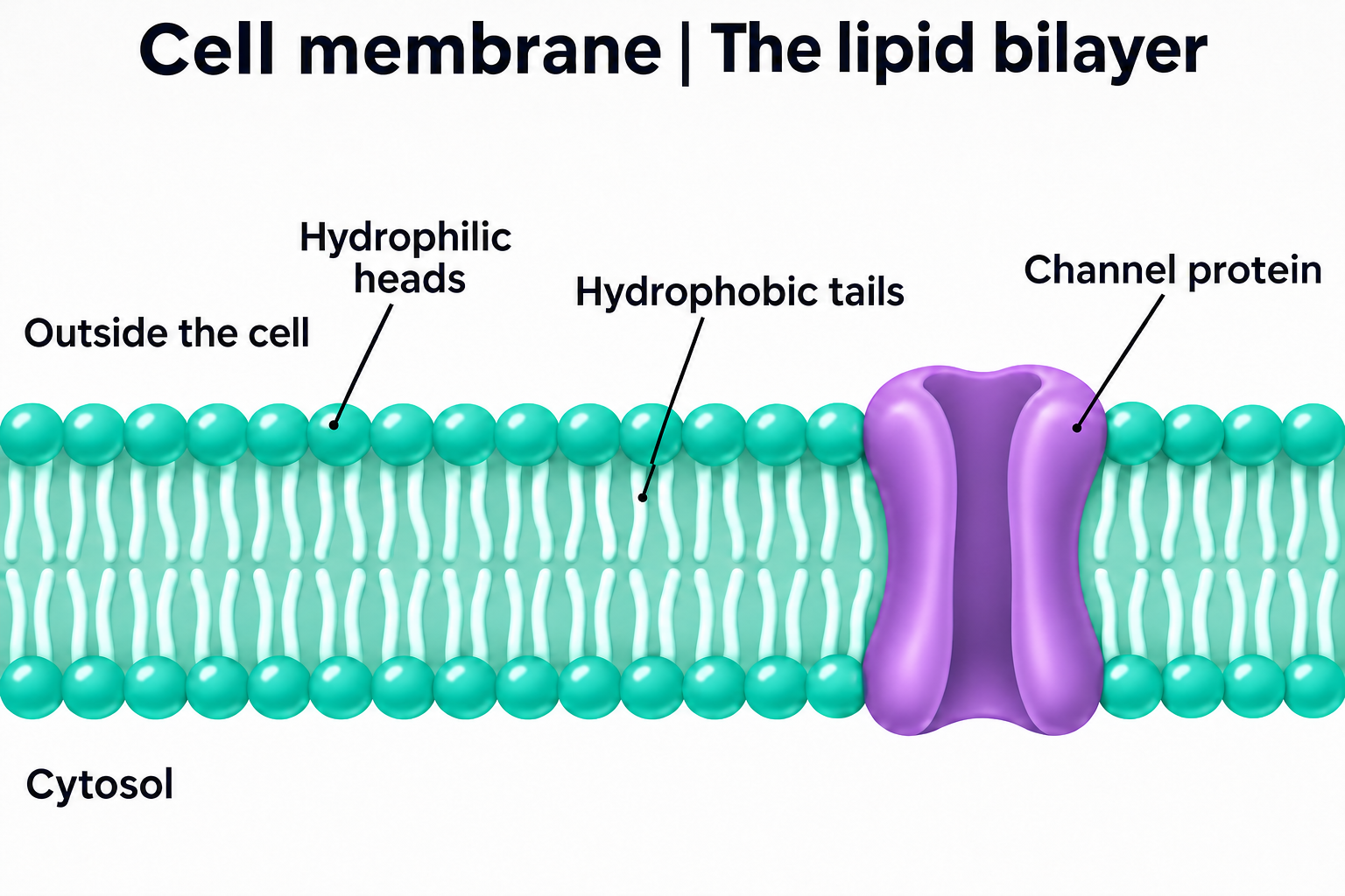
The lipid bilayer
Introduce the arrangement of phospholipids in a cell membrane.

The fluid mosaic model
Explore the proteins and lipids shown in a fluid mosaic membrane model.


A molecular landscape
A detailed membrane view for discussing its molecular organisation.

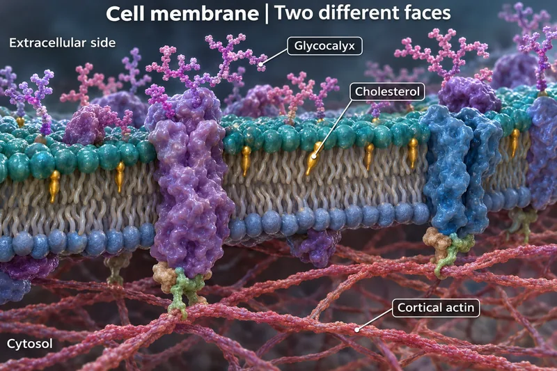
Two different faces
Compare the extracellular surface with the cytosolic side of this membrane.


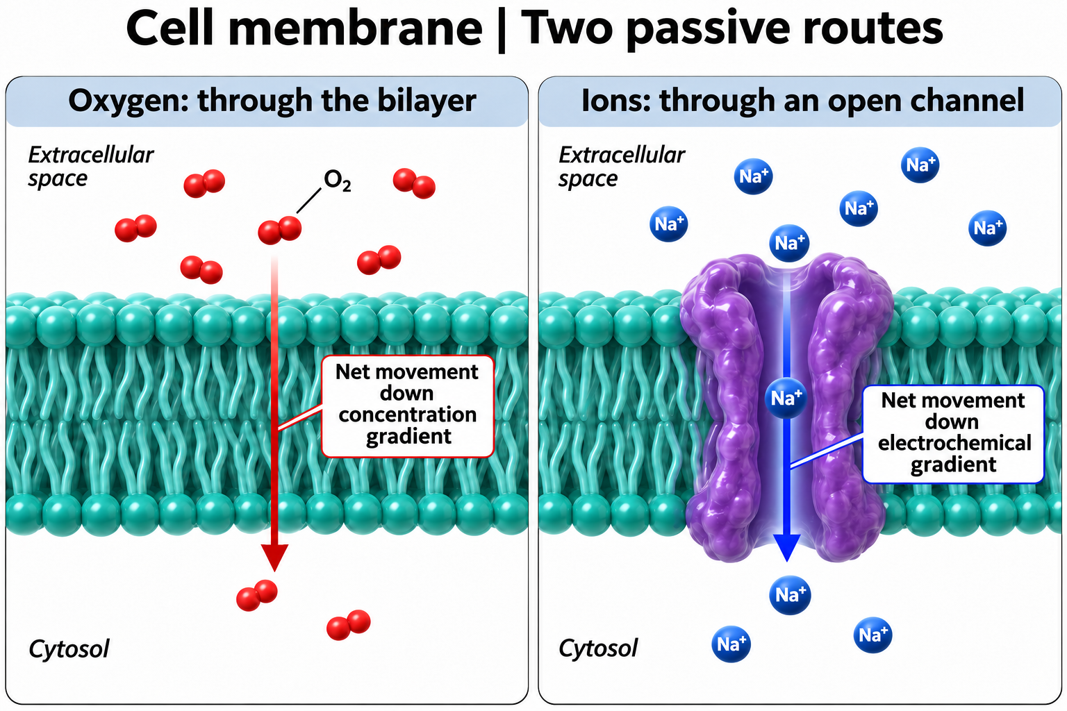
Two passive routes
Compare oxygen diffusion through the bilayer with ion movement through an open channel.
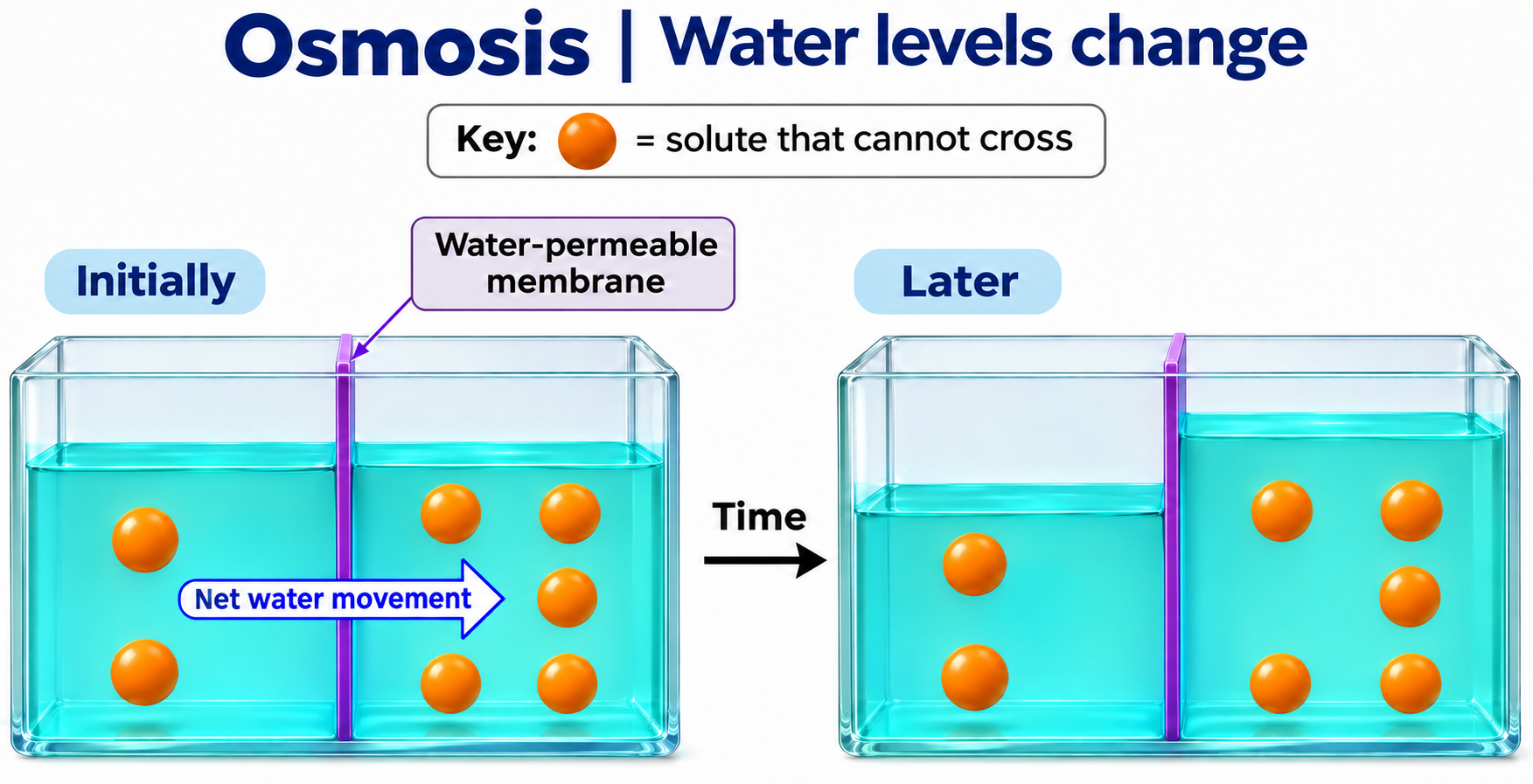
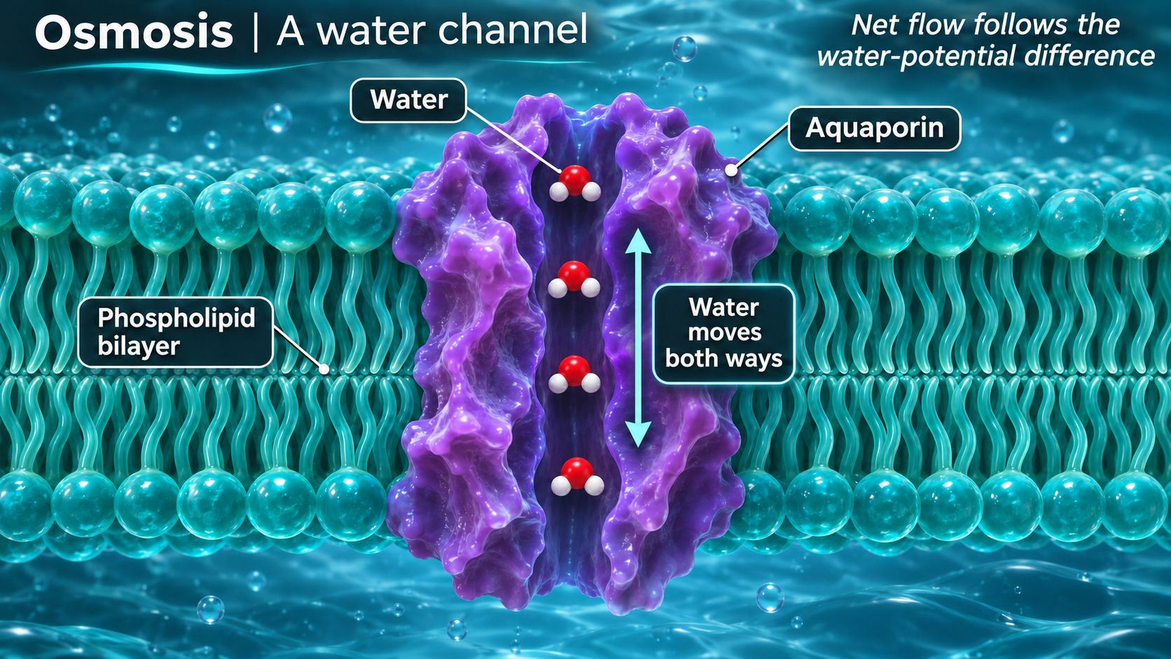
 BIOLOGY · 5 VISUALSOsmosisExplore water movement, water channels, pressure and red blood cells.
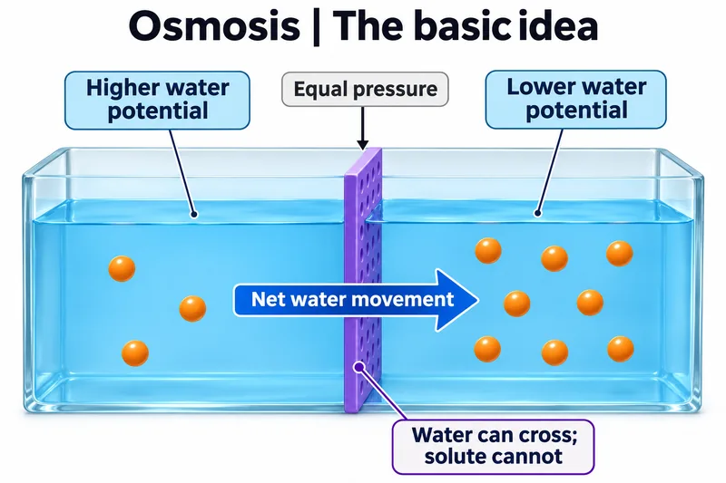
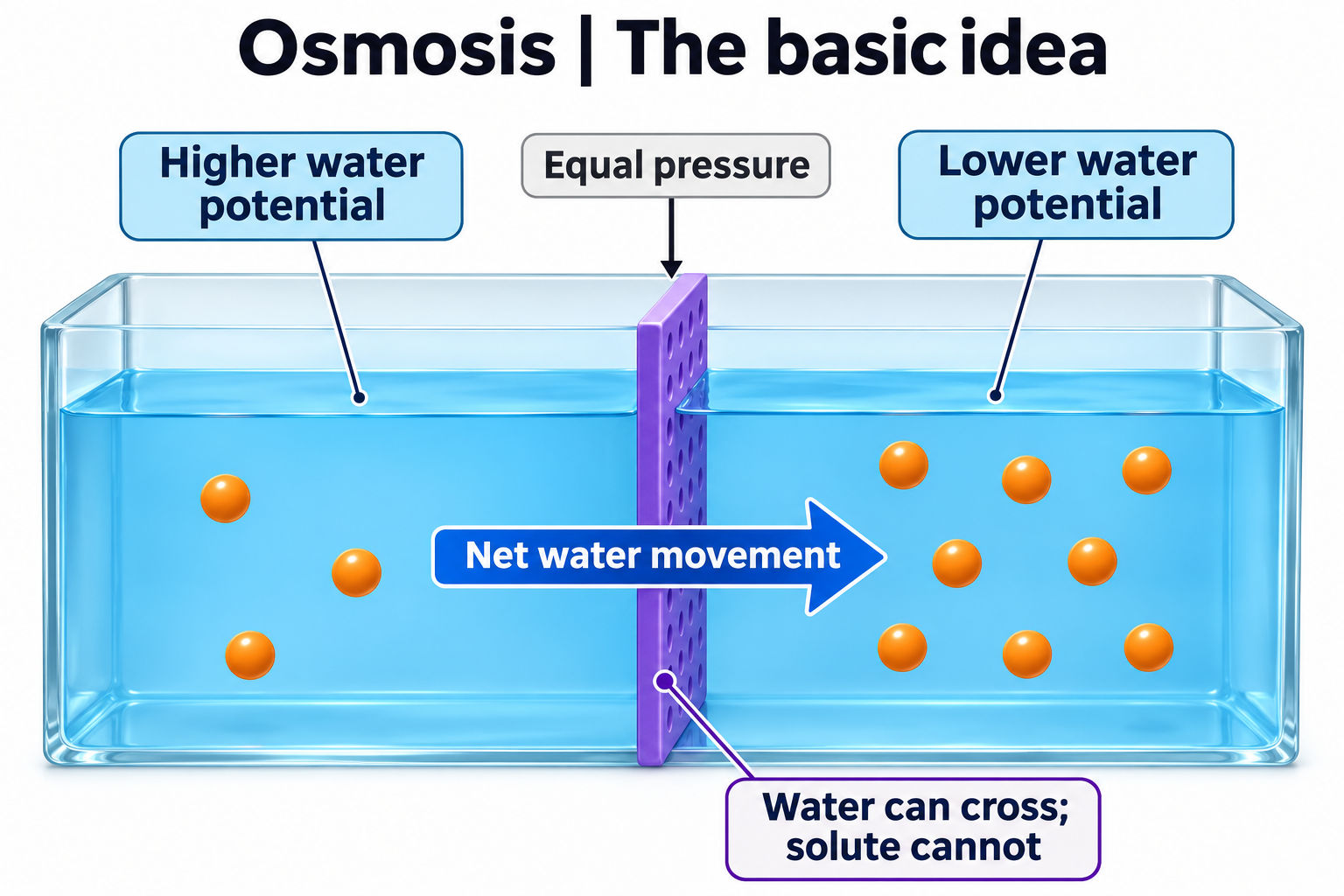
The basic idea
Introduce net water movement across a selectively permeable membrane.

Water levels change
Compare initial water levels with the levels after net water movement.

Through a water channel
Explore water movement through a membrane channel.

Pressure matters
Use the example values to discuss pressure and solute potential at equilibrium.

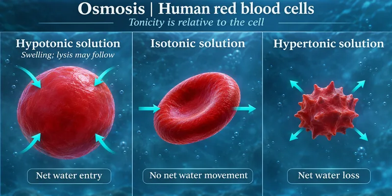
Red blood cells
Compare red blood cells in solutions with different tonicities.

 BIOLOGY · 5 VISUALSFacilitated diffusionExplore channels, carrier proteins, alternating access and transport selectivity.
Through a channel
Follow ion movement through a channel down its electrochemical gradient.


Two protein routes
Compare channel-mediated ion transport with carrier-mediated glucose transport without ATP use.


A carrier changes shape
Follow glucose binding, occlusion and release as a carrier changes conformation.


Carrier saturation
Explore how a fixed number of carriers limits glucose uptake as concentration rises.

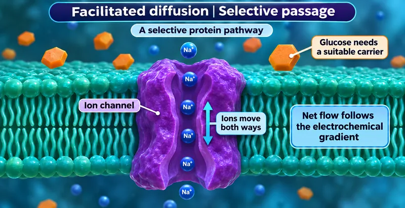
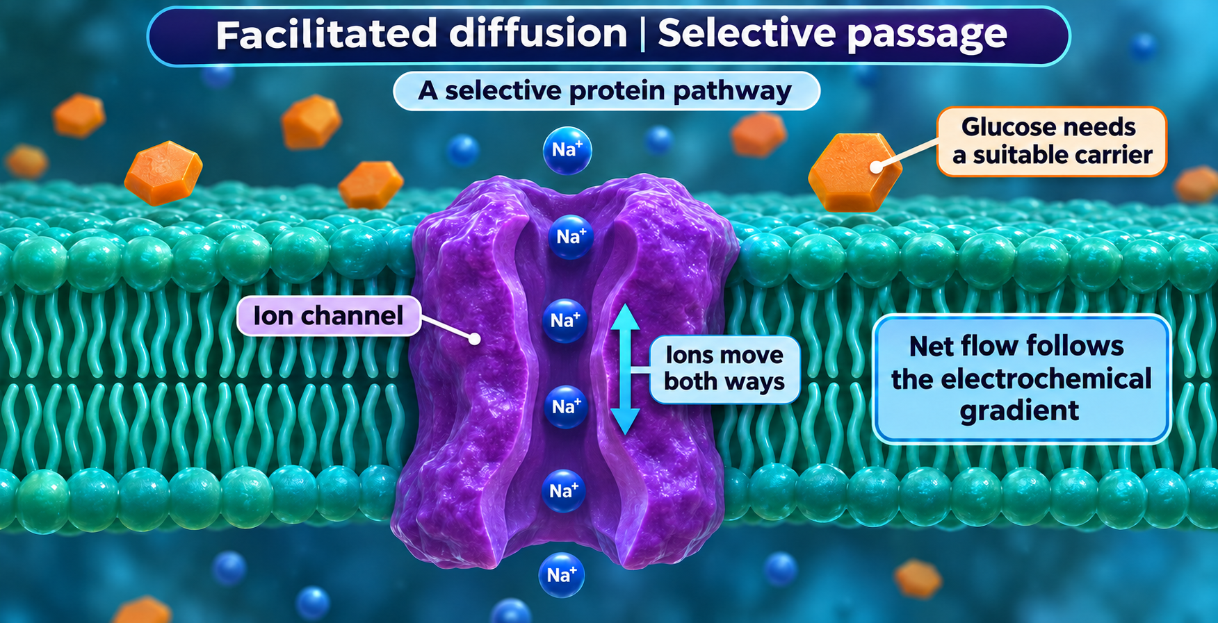
Selective passage
Compare a selective protein pathway with glucose transport through a suitable carrier.
 BIOLOGY · 5 VISUALSSodium potassium pumpExplore ATP-driven sodium and potassium transport across a cell membrane.
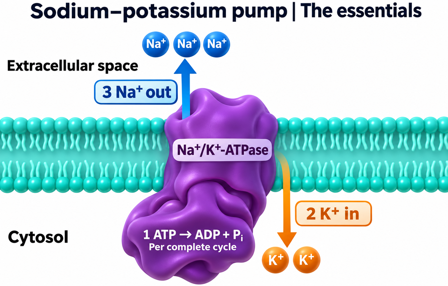
The essentials
Follow three sodium ions out and two potassium ions in per ATP hydrolysed.

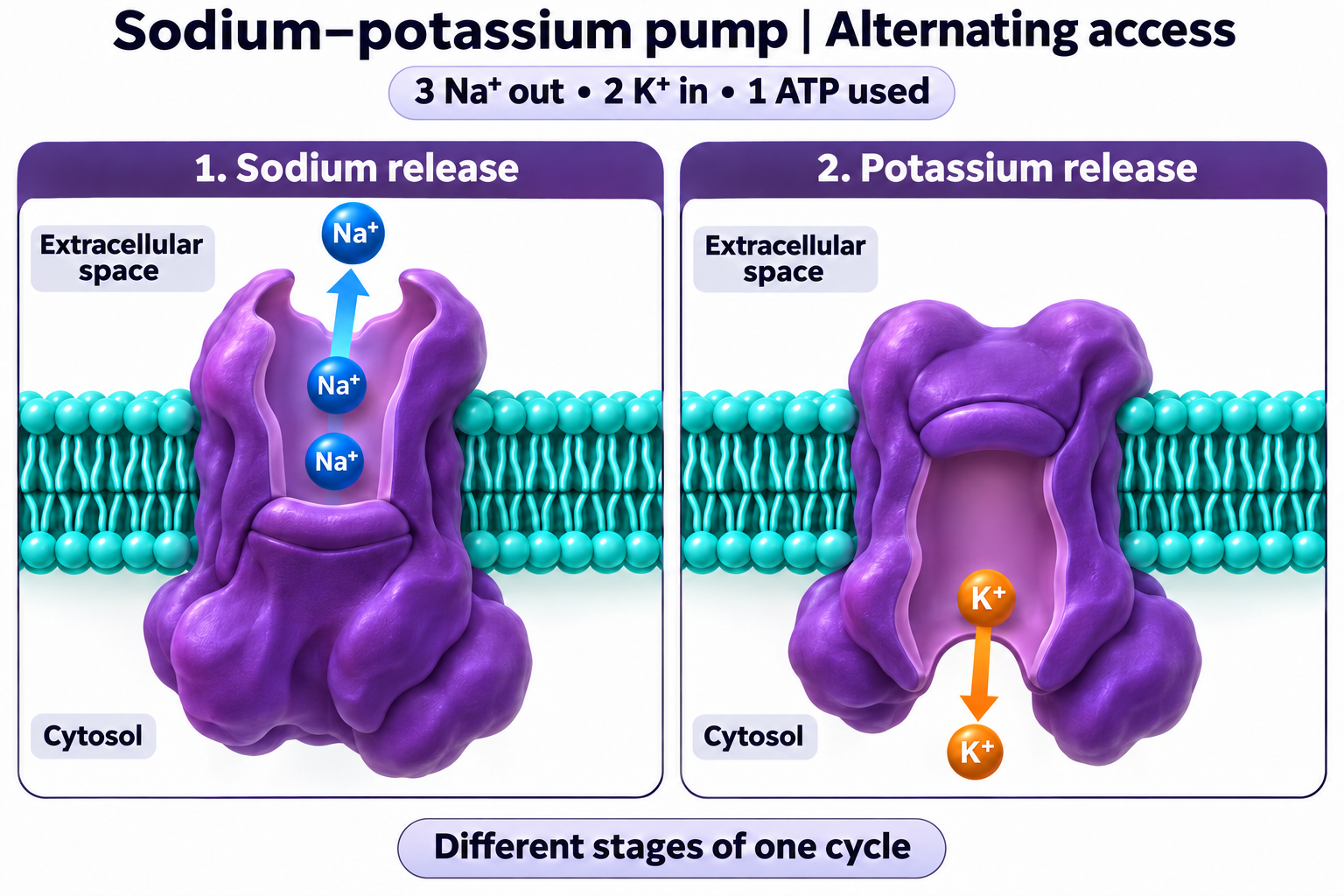
Alternating access
Compare sodium-release and potassium-release stages of one pump cycle.

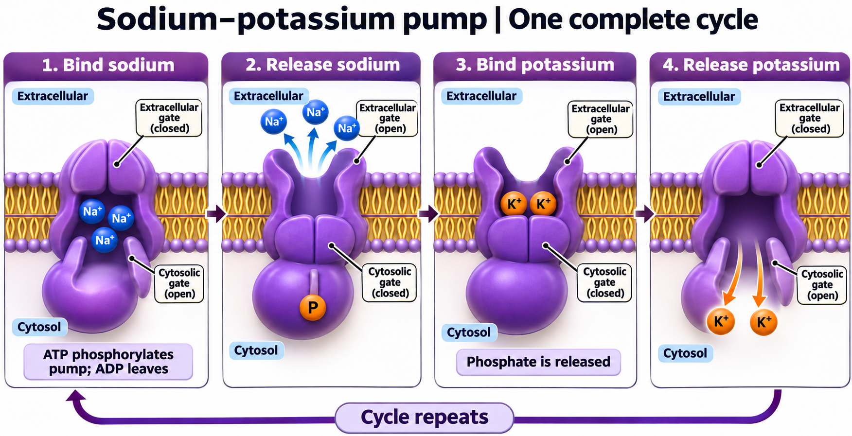
One complete cycle
Follow sodium binding and release, potassium binding and release, and pump phosphorylation.

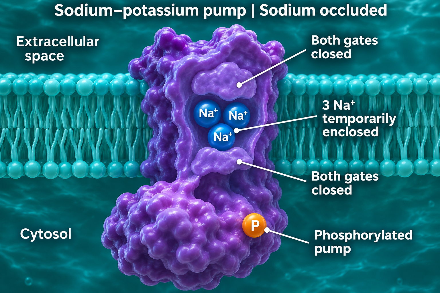
Sodium occluded
View the phosphorylated pump with three sodium ions enclosed and both gates closed.

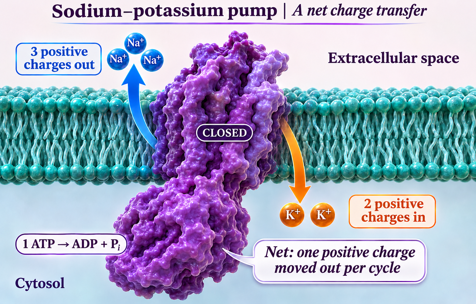
A net charge transfer
Compare three positive charges moving out with two moving in: one net positive charge leaves per cycle.
 BIOLOGY · 5 VISUALSMitochondrionExplore realistic illustrative views of mitochondrial membranes and cristae.
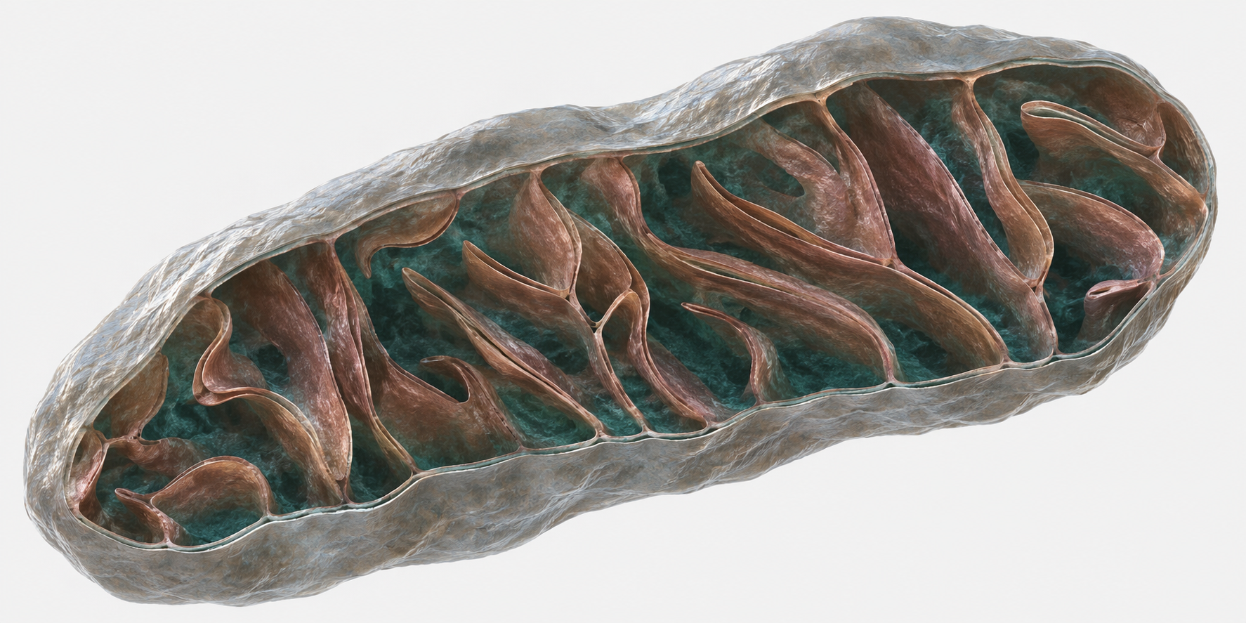
Whole organelle
Explore a realistic illustrative cutaway of the mitochondrial envelope and cristae.

Labelled ultrastructure
Locate the membranes, matrix and folded cristae in a labelled mitochondrial illustration.

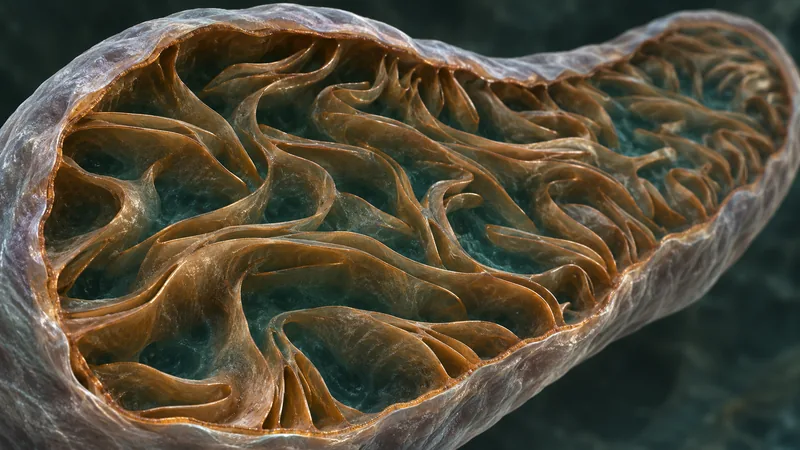
Oblique interior
Inspect cristae from an oblique cutaway view inside a mitochondrion.

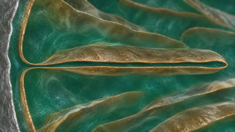
Crista junction
Explore the narrow connection between a crista and the inner boundary membrane.
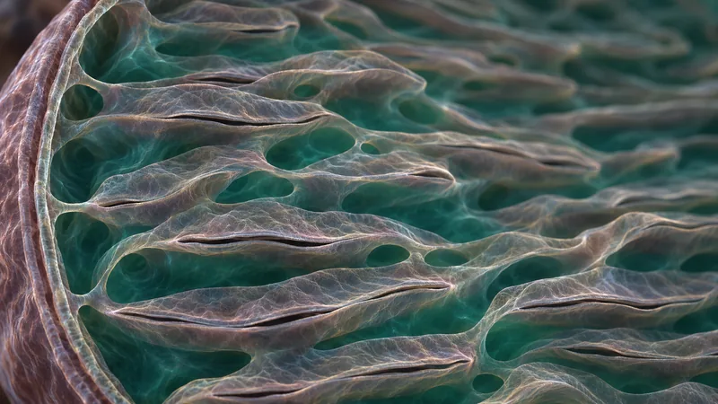
Lamellar detail
Examine the layered arrangement of lamellar cristae in an illustrative close-up.
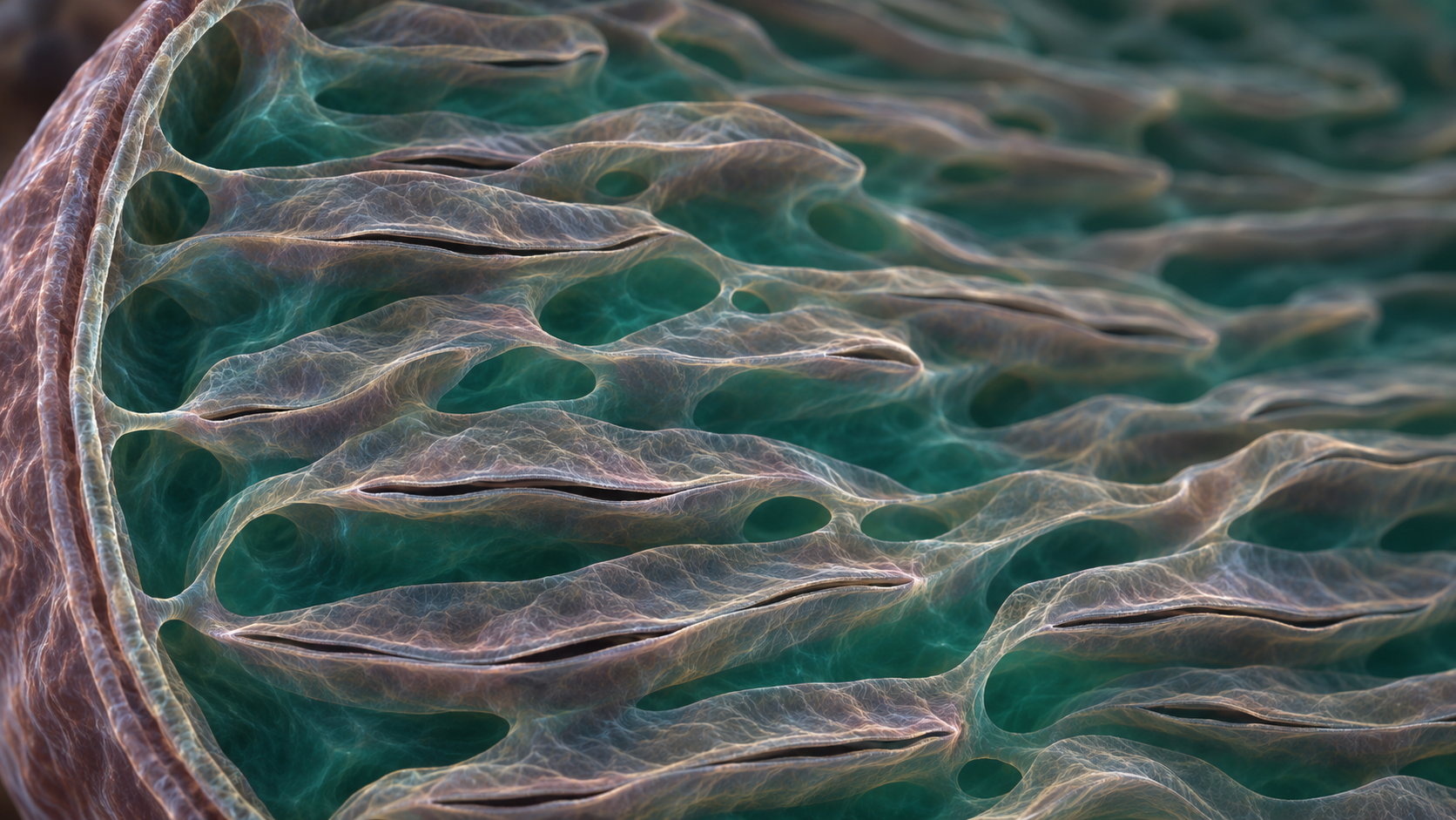
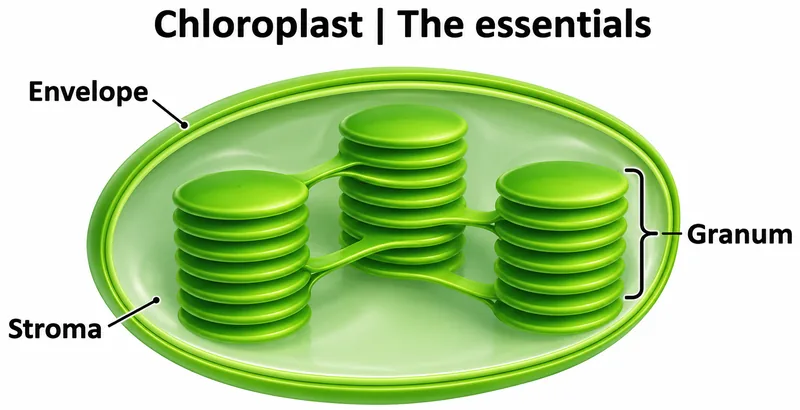 BIOLOGY · 5 VISUALSChloroplastExplore chloroplast structure, thylakoid connections and photosynthesis locations.
The essentials
Locate the envelope, stroma and internal membrane stacks of a chloroplast.


Inside the organelle
Explore the chloroplast envelope, grana and stroma lamellae.


Connected thylakoids
Explore connections between thylakoid membranes and their internal lumen.


Making ATP
Explore ATP production associated with the thylakoid membrane.


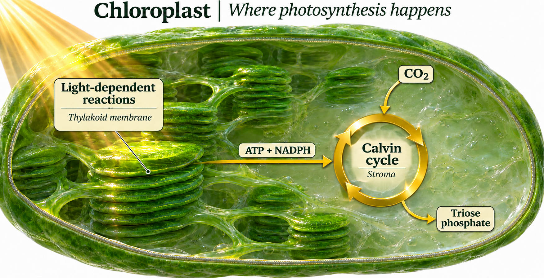
Where photosynthesis happens
Locate light-dependent reactions at thylakoid membranes and carbon fixation in the stroma.
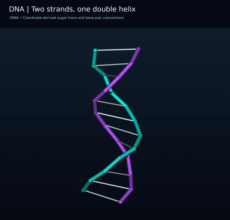 BIOLOGY · 5 VISUALSDNAExplore coordinate-based molecular representations from the 1BNA DNA structure.
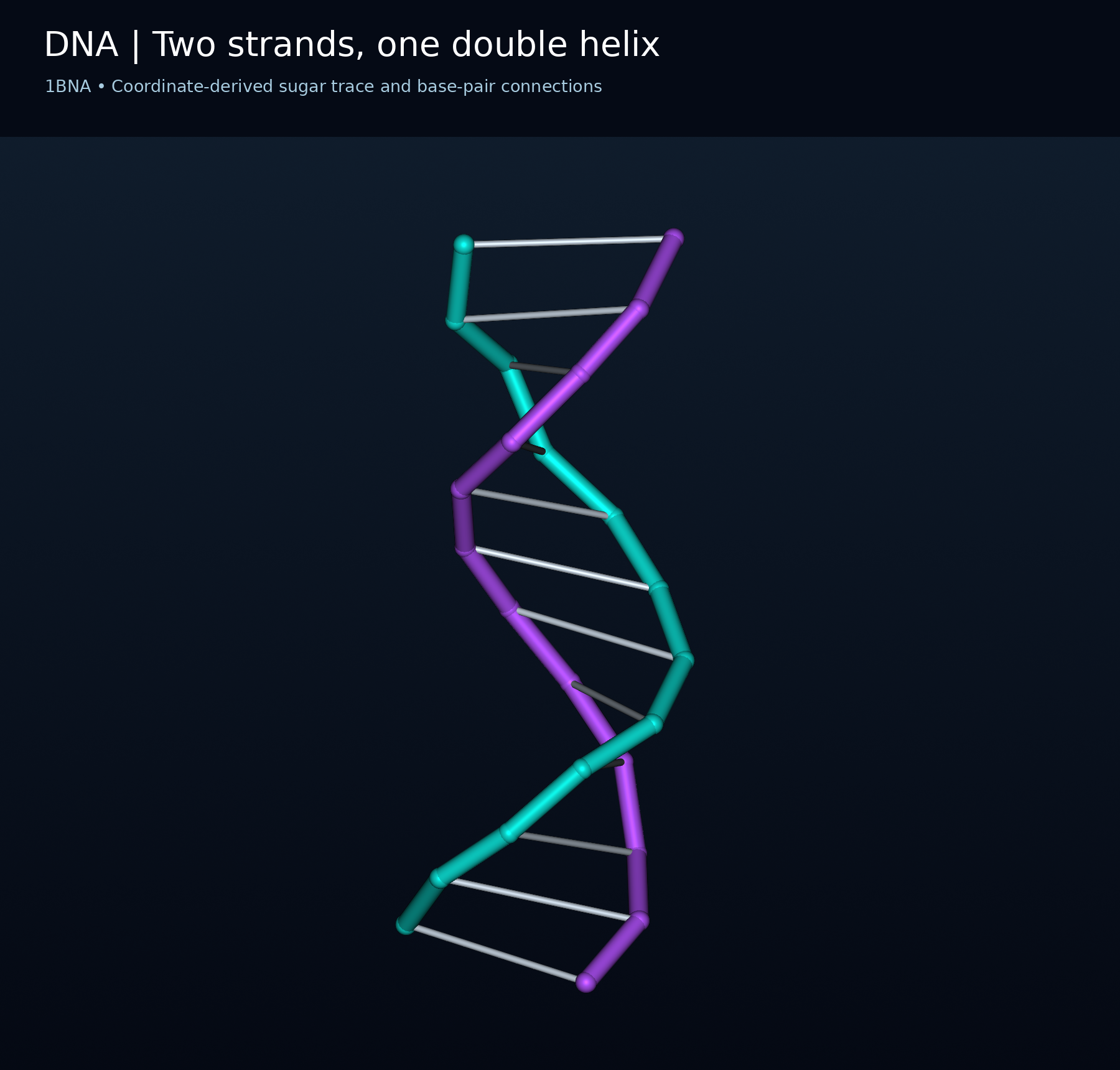
Two strands, one double helix
Coordinate-derived sugar trace and base-pair connections from DNA structure 1BNA.

The atomic framework
Deposited non-hydrogen atoms of 1BNA, with the two DNA chains coloured separately.


Atoms and covalent connections
A 1BNA atom-and-bond view with carbon, nitrogen, oxygen and phosphorus distinguished by colour.


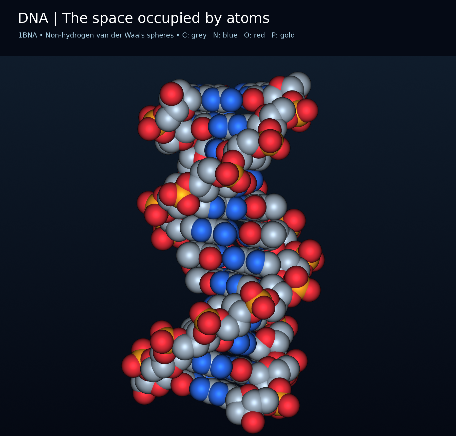
The space occupied by atoms
Non-hydrogen van der Waals spheres rendered from 1BNA coordinates.

An adenine-thymine pair
Base atoms of 1BNA residues A6 and T19; hydrogen atoms and hydrogen-bond lines are omitted.

 BIOLOGY · 5 VISUALSDNA replicationFollow semiconservative replication, strand synthesis and fragment joining.
One old strand in each copy
Semiconservative replication leaves one parental strand in each new DNA molecule.


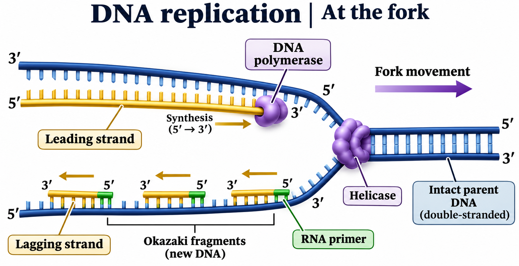
At the fork
Leading and lagging strands, helicase, primers and 5′ to 3′ DNA synthesis.
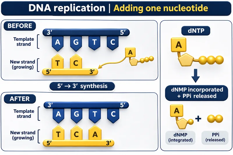
Adding one nucleotide
A complementary nucleotide joins the growing strand, with pyrophosphate released.

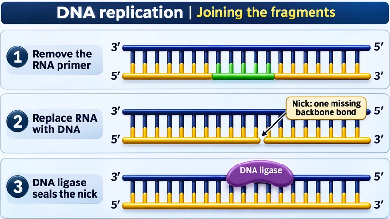
Joining the fragments
Primer removal, DNA replacement and ligase sealing a remaining nick.

Opening the double helix
An illustrative view of helicase and single-strand binding proteins at a replication fork.

 BIOLOGY · 5 VISUALSTranscription and translationFollow the message from DNA to RNA and a growing polypeptide.
DNA to protein
Transcription in a eukaryotic nucleus, mRNA export and translation at a ribosome.

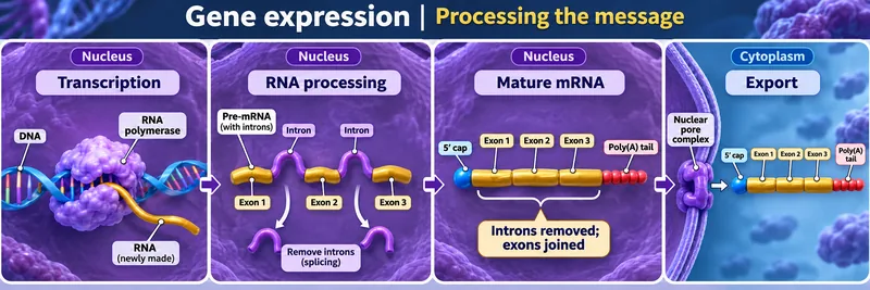
Processing the message
Pre-mRNA processing removes introns, joins exons and prepares mRNA for export.


Reading a codon
The AUG codon pairs with a UAC anticodon on a methionine-carrying tRNA.


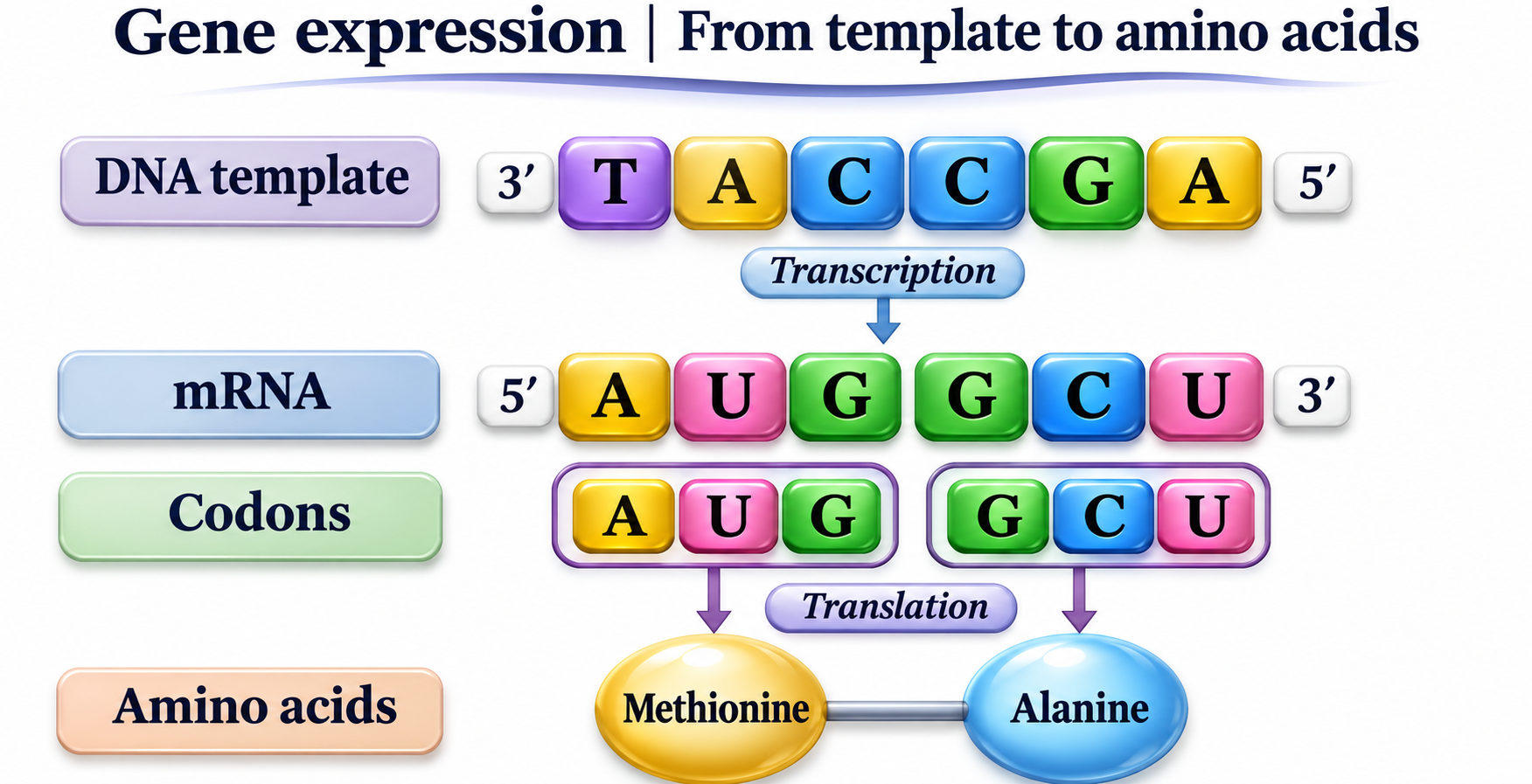
From template to amino acids
A short DNA template is transcribed into mRNA codons for methionine and alanine.

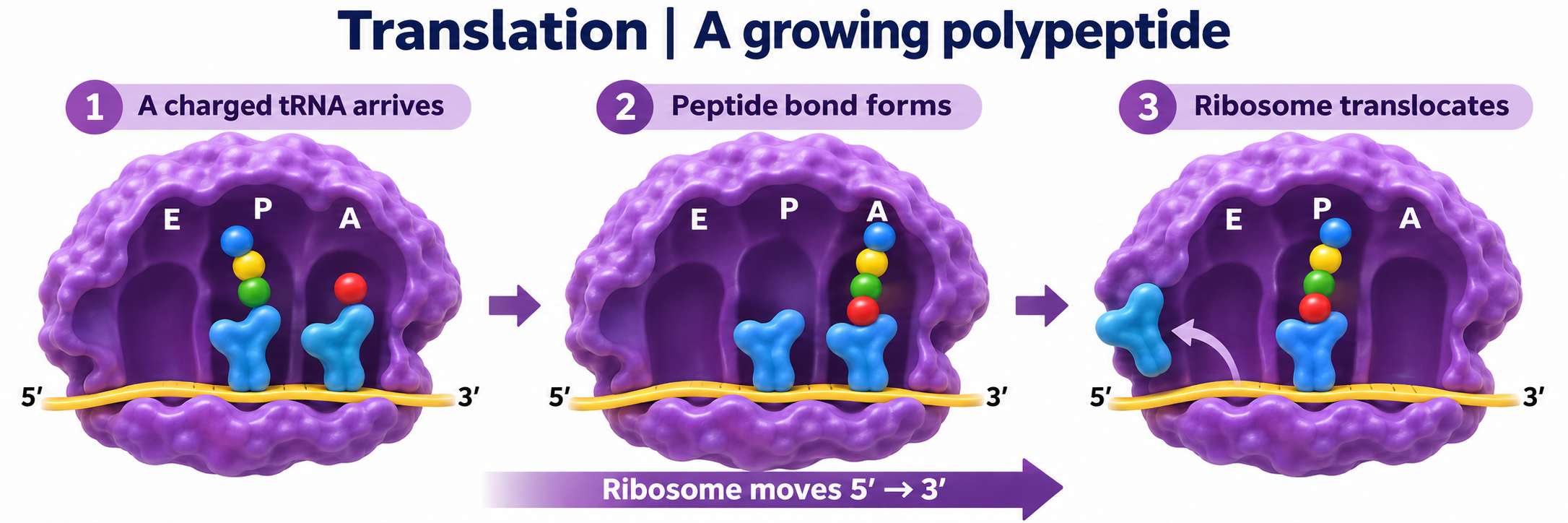
A growing polypeptide
A charged tRNA arrives, a peptide bond forms and the ribosome translocates.
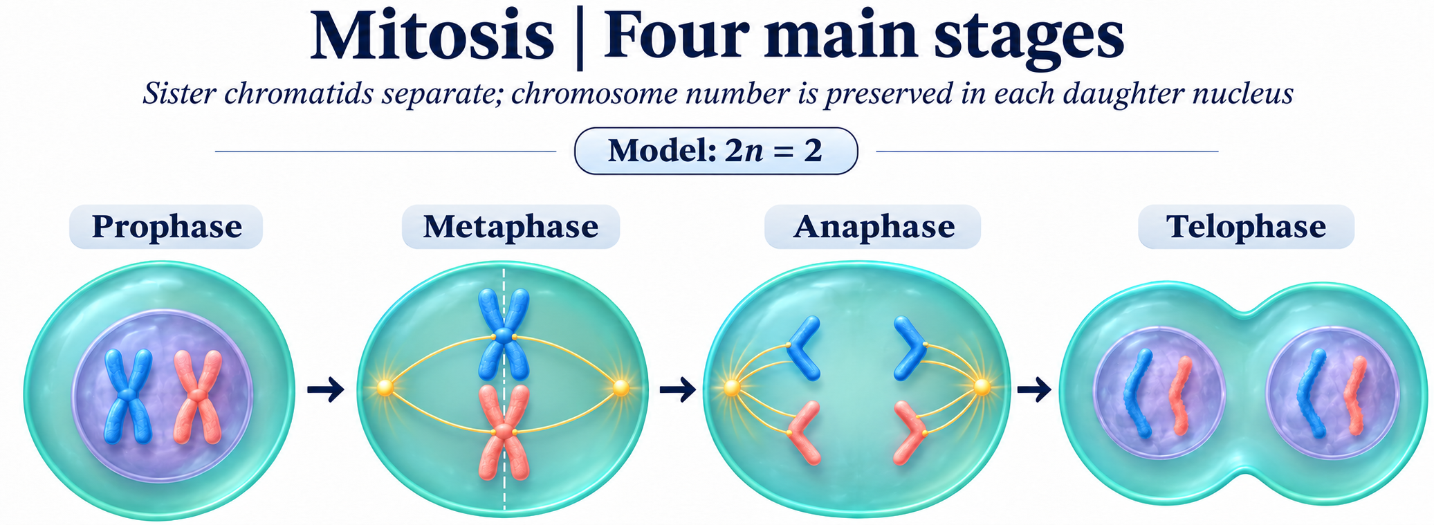
 BIOLOGY · 5 VISUALSMitosisExplore chromosome separation and division using a simplified chromosome model.
Four main stages
Prophase, metaphase, anaphase and telophase in a simplified 2n = 2 model.

Metaphase attachment
Sister chromatids, kinetochores, spindle poles and the equatorial plane.


One chromosome, two daughters
Track sister chromatids as they separate into daughter chromosomes.


Cytokinesis
A cleavage furrow and contractile ring divide an animal cell after chromosome separation.


DNA copied, then shared
Compare chromosome and DNA-molecule counts before replication and after division.

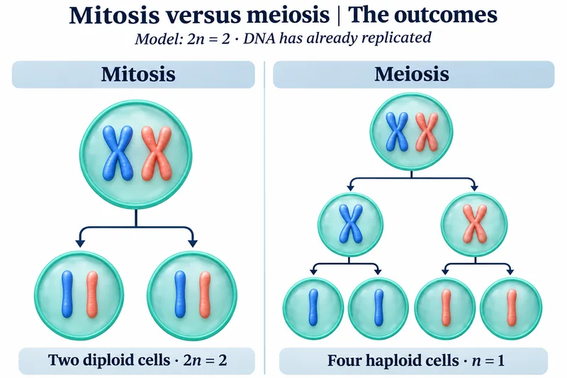 BIOLOGY · 5 VISUALSMitosis versus meiosisCompare outcomes, chromosome separation and sources of genetic variation.
The outcomes
Two diploid products of mitosis compared with four haploid products of meiosis.


What separates?
Sisters separate in mitosis and meiosis II; homologues separate in meiosis I.


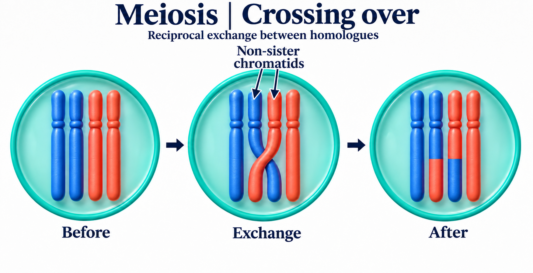
Crossing over
Reciprocal exchange between non-sister chromatids of homologous chromosomes.
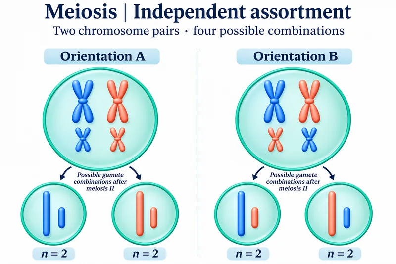
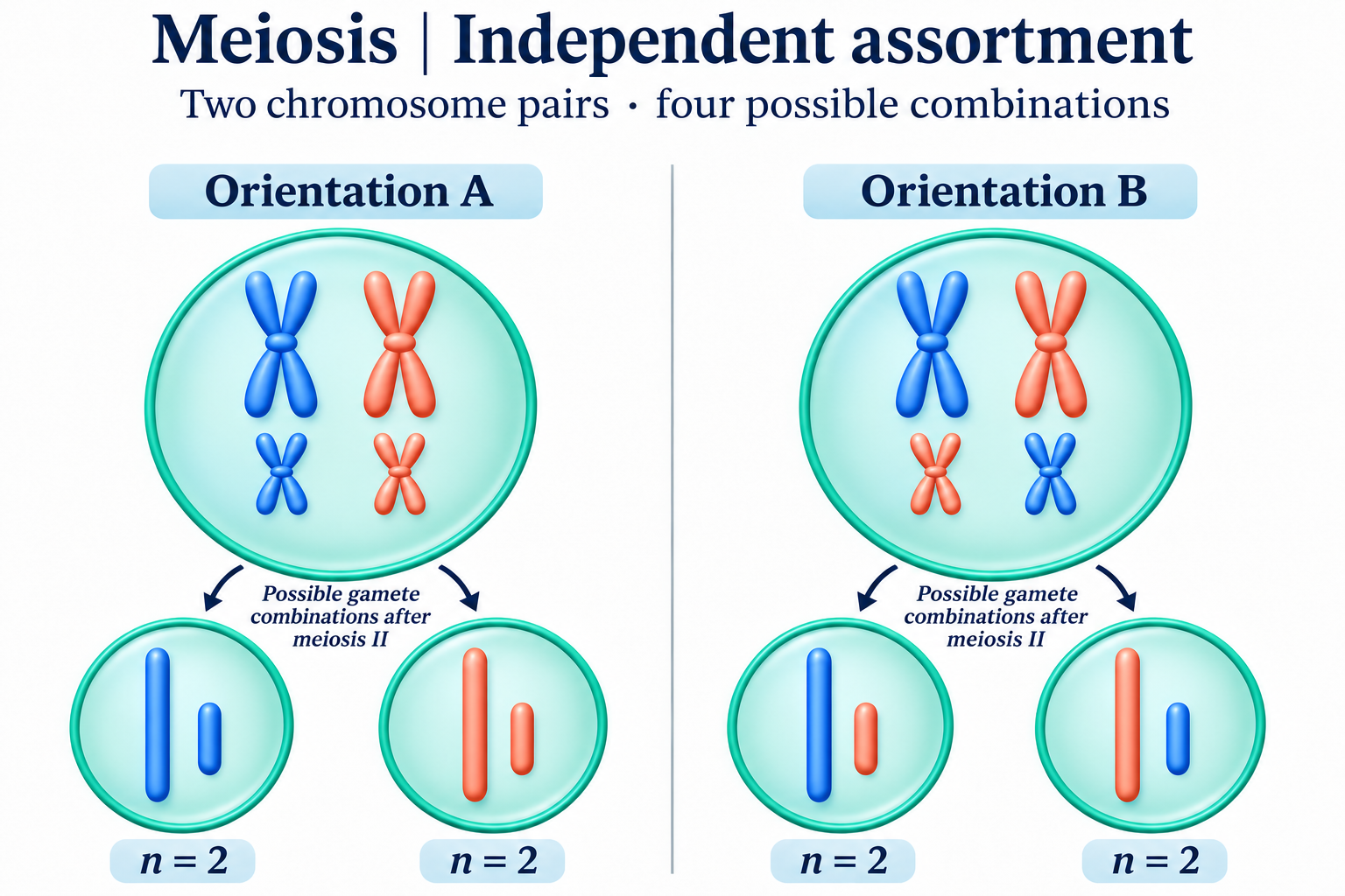
Independent assortment
Two chromosome pairs illustrate alternative orientations and four gamete combinations.

Division and DNA
Track chromosome sets and DNA amount through mitosis and both meiotic divisions.

 BIOLOGY · 5 VISUALSEnzyme shape and bindingExplore binding illustrations and deposited adenylate kinase structures.
Binding changes shape
A conceptual sequence of substrate binding, active-site adjustment and product release.


A flexible active site
An illustrative comparison before binding and in the bound complex.


Competing for the active site
Compare substrate binding with a competitive inhibitor occupying the active site.


Open and closed states
E. coli adenylate kinase structures 4AKE and 1AKE, chain A; the closed model contains Ap5A inhibitor. Static structures, not a time sequence.


The occupied cleft
A surface representation of adenylate kinase 1AKE, chain A, with Ap5A inhibitor shown in yellow.

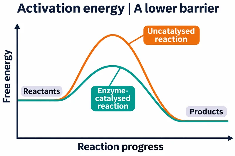 BIOLOGY · 5 VISUALSActivation energyQualitative energy profiles explain catalysis, rates and equilibrium.
A lower barrier
Catalysed and uncatalysed pathways share reactant and product energies.


Reading the profile
Compare activation barriers while keeping the overall free-energy change unchanged.


Both directions accelerate
An enzyme lowers forward and reverse activation barriers.

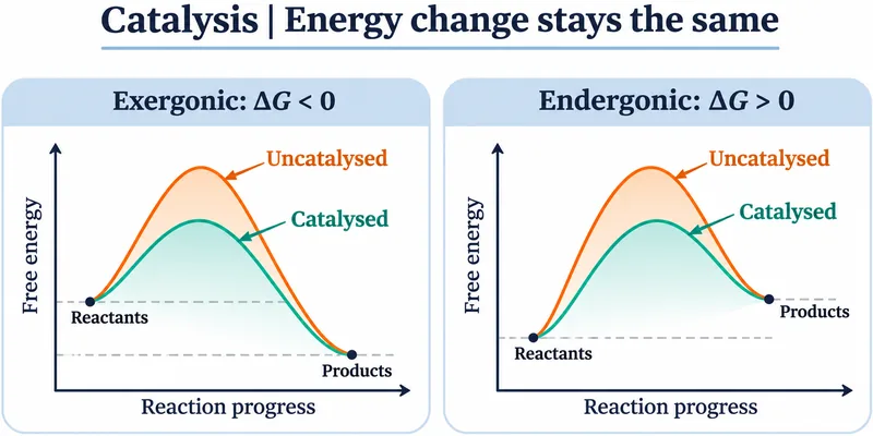
Energy change stays the same
Catalysis in exergonic and endergonic reactions does not alter the overall energy change.


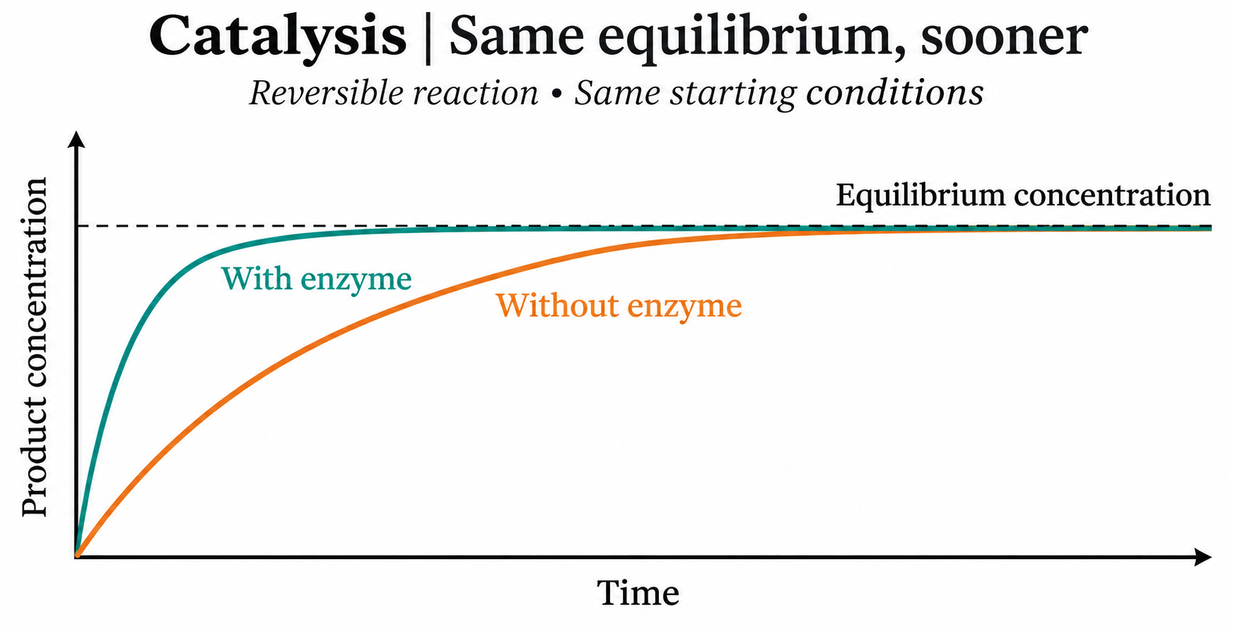
Same equilibrium sooner
Qualitative concentration curves approach the same equilibrium with and without enzyme.
 BIOLOGY · 5 VISUALSPhotosynthesis overviewConnect light reactions, the Calvin cycle and the origin of released oxygen.
The big picture
Sunlight, water and carbon dioxide support carbohydrate production and oxygen release.


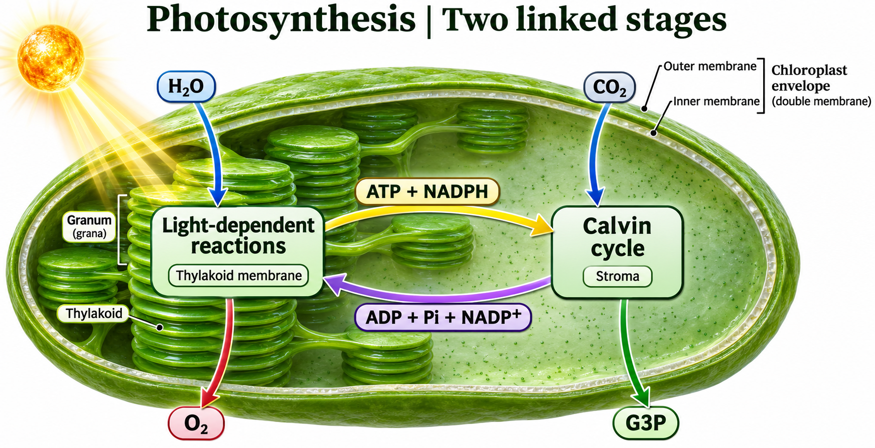
Two linked stages
Light reactions supply ATP and NADPH to the Calvin cycle in the chloroplast.
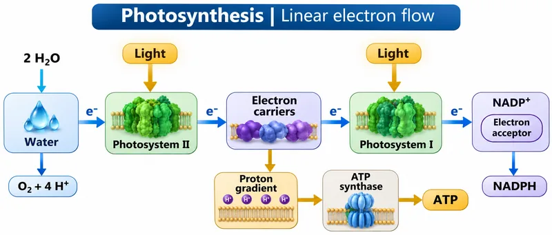
Linear electron flow
Follow electrons from water through photosystems II and I to NADPH.

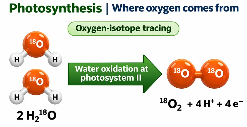
Where oxygen comes from
Oxygen-isotope tracing illustrates water as the source of released oxygen.


The proton gradient
An illustrative thylakoid membrane shows proton transfer and return through ATP synthase.

 BIOLOGY · 5 VISUALSCalvin cycleFollow carbon fixation, reduction, regeneration and the energy budget.
Three phases
Fixation, reduction and regeneration in the chloroplast stroma.


Molecules in motion
Three CO2 enter the cycle and one G3P is the net carbon product.


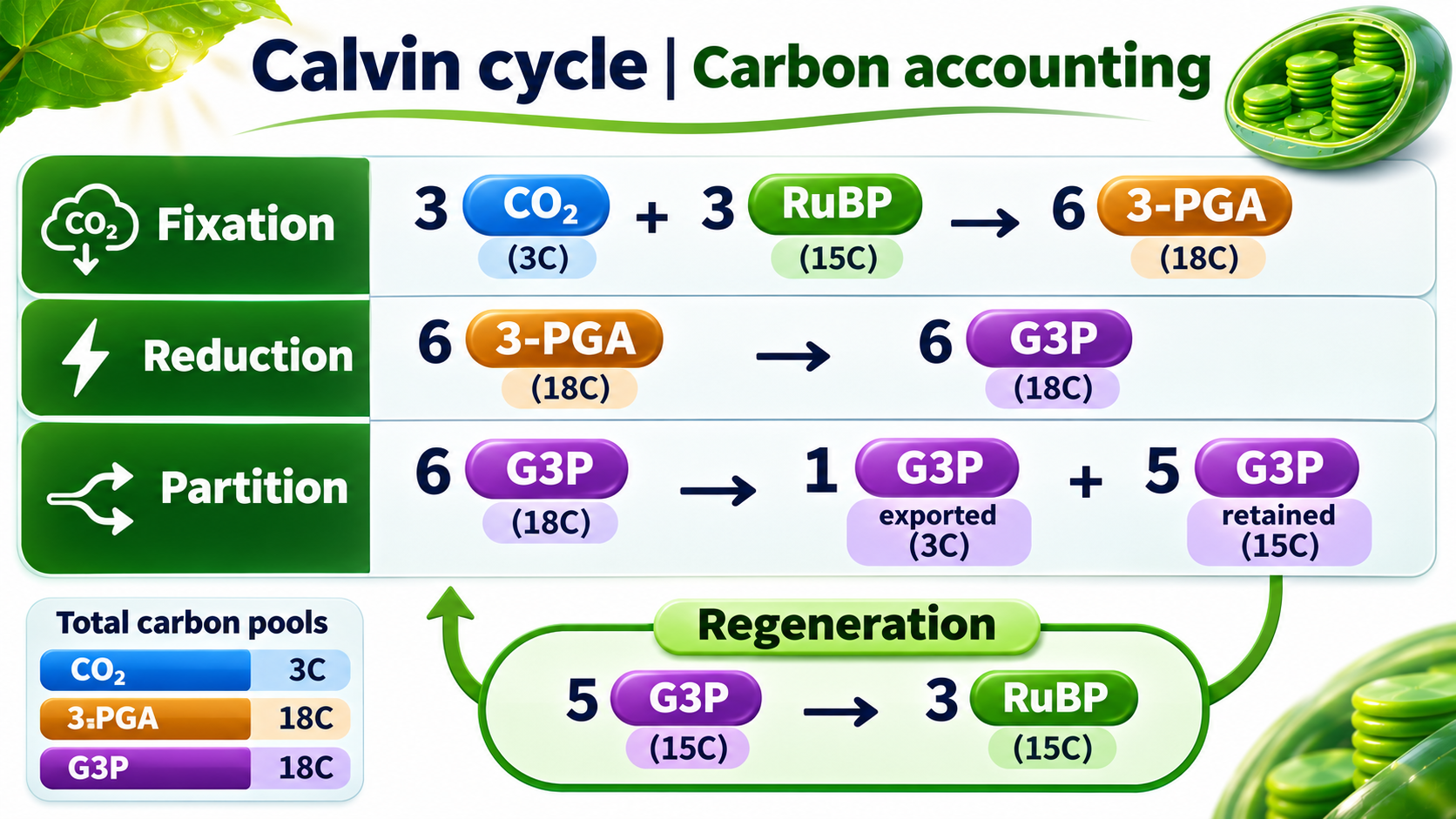
Carbon accounting
Track carbon totals through fixation, G3P partition and RuBP regeneration.

The energy budget
One net G3P from three CO2 requires nine ATP and six NADPH.

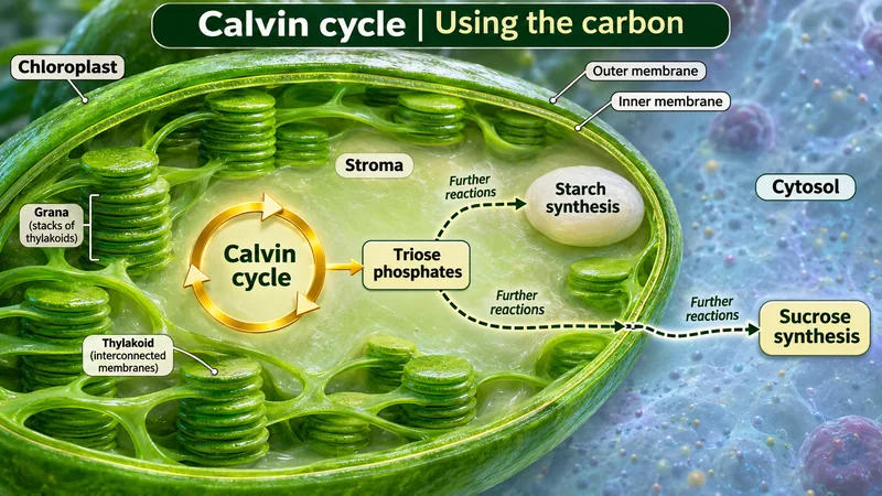
Using the carbon
Triose phosphates support starch synthesis in the chloroplast and sucrose synthesis in the cytosol.

 BIOLOGY · 5 VISUALSGlycolysisTrack carbon and energy from glucose to pyruvate in the cytosol.
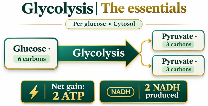
The essentials
One glucose yields two pyruvate, a net two ATP and two NADH.

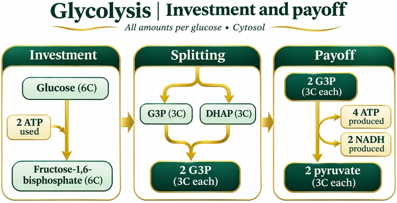
Investment and payoff
Two ATP are invested before the pathway produces four ATP and two NADH.

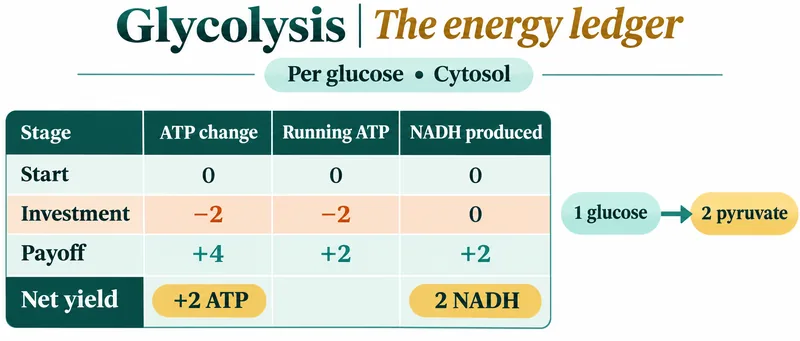
The energy ledger
A per-glucose ledger separates ATP investment, payoff and net yield.


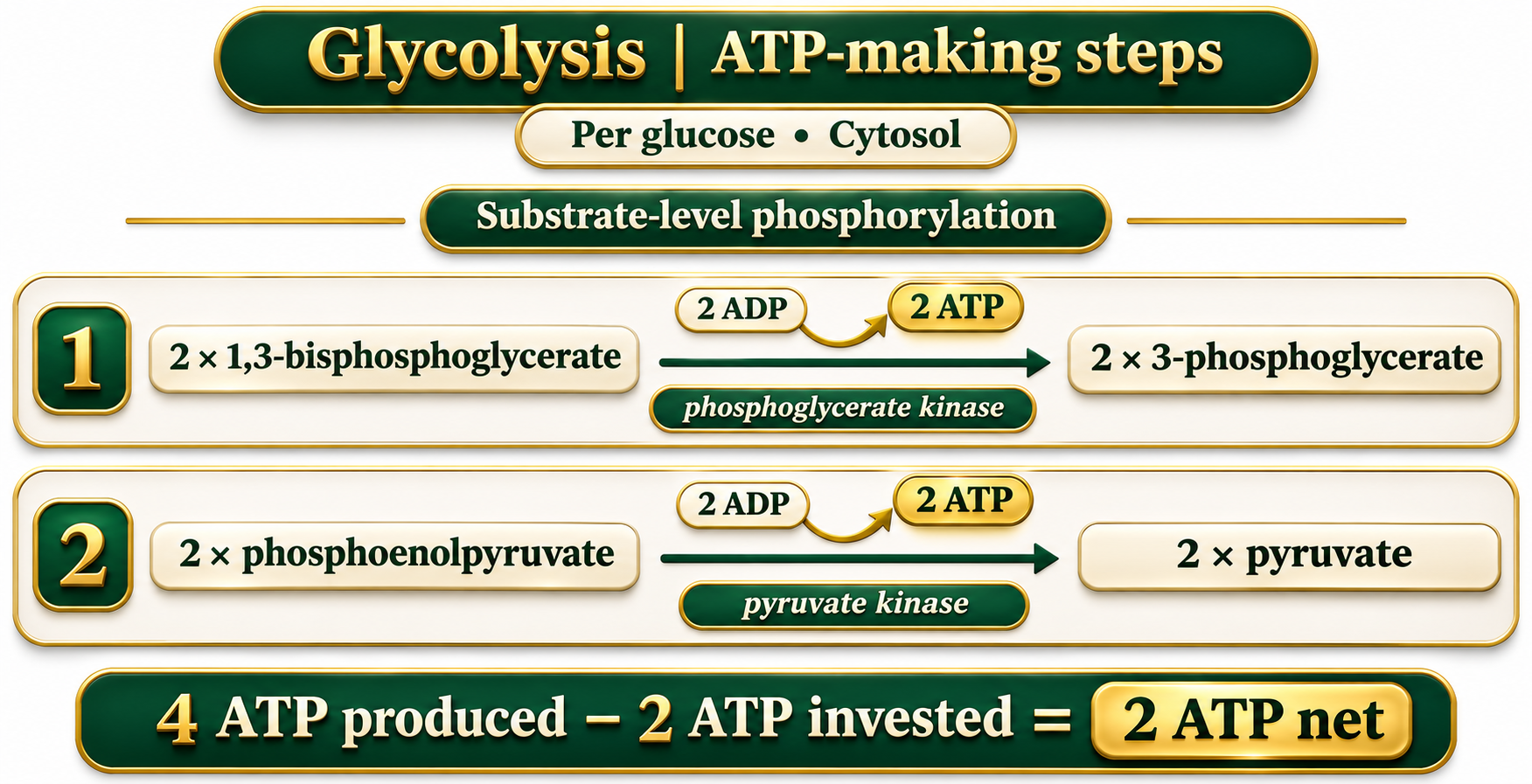
ATP-making steps
Substrate-level phosphorylation at phosphoglycerate kinase and pyruvate kinase steps.

Carbon accounting
Six carbons enter as glucose and leave in two pyruvate; symbols count carbons, not molecular geometry.

 BIOLOGY · 5 VISUALSCitric acid cycleExplore carbon flow and carrier production in a GTP-forming route.
One turn
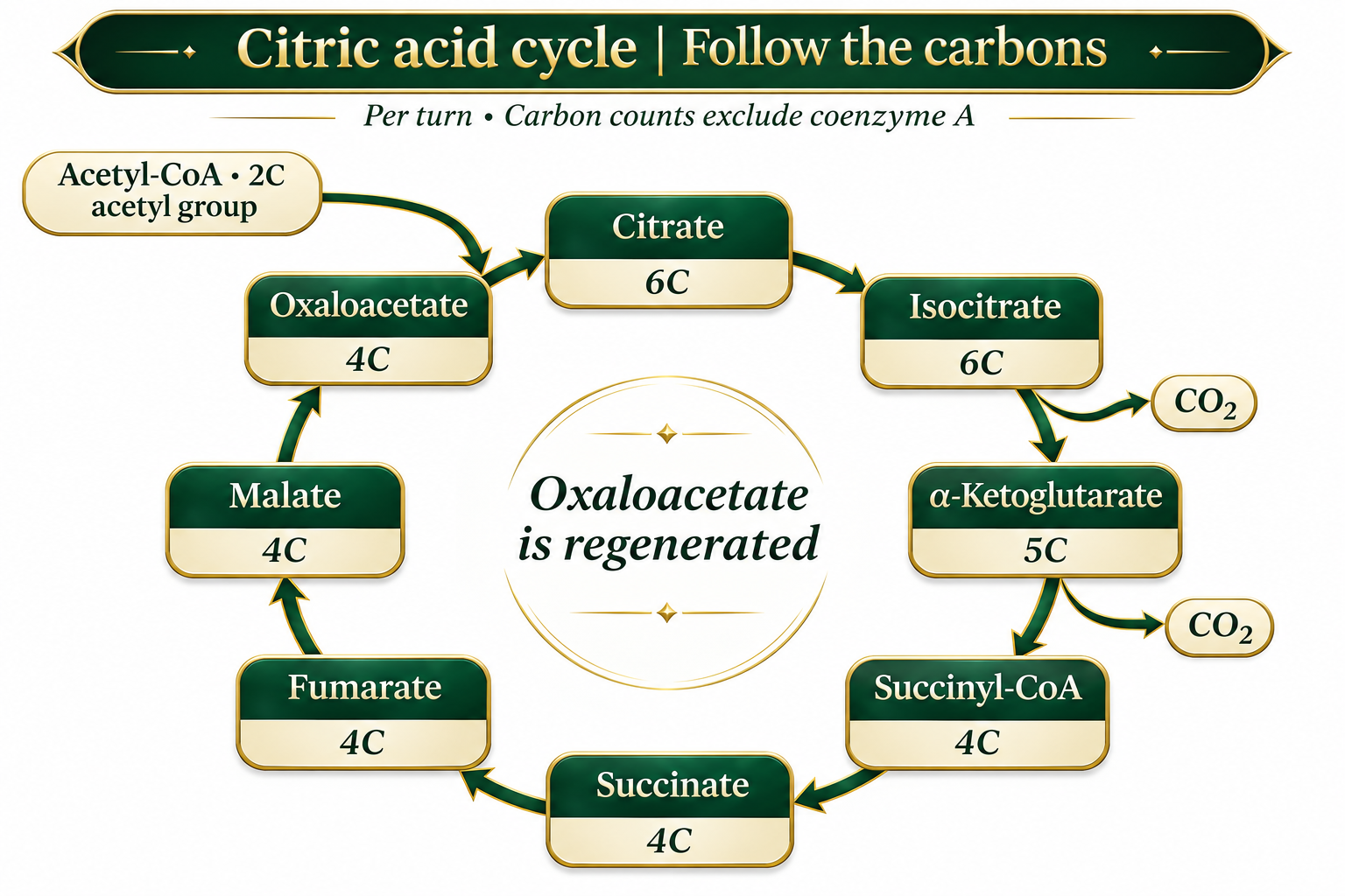
Per acetyl-CoA: two CO2, three NADH, one FADH2 equivalent and one GTP.


Follow the carbons
Track carbon counts through cycle intermediates and oxaloacetate regeneration.

Where carriers form
Carrier-forming reactions, including reduction of enzyme-bound FAD at succinate dehydrogenase.


The link reaction
Distinguish pyruvate oxidation from the citric acid cycle that follows.

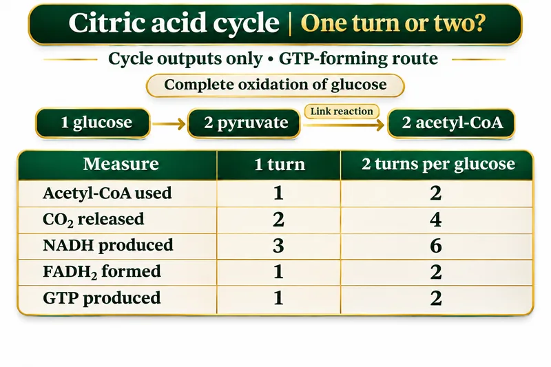
One turn or two?
Compare cycle-only outputs per acetyl-CoA and per glucose; the illustrated route produces GTP.

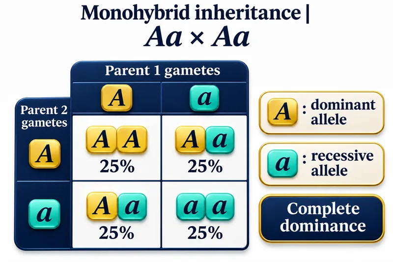 BIOLOGY · 5 VISUALSMonohybrid inheritanceExplore inheritance probabilities for an Aa × Aa cross with complete dominance.
A Punnett square
Four equally likely combinations give AA, Aa, Aa and aa.
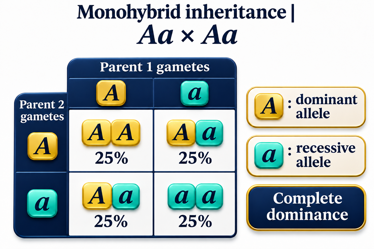

From parents to gametes
Each heterozygous parent contributes either allele with probability one half.


Two independent contributions
A probability tree combines the two parental allele contributions.


Genotype and phenotype
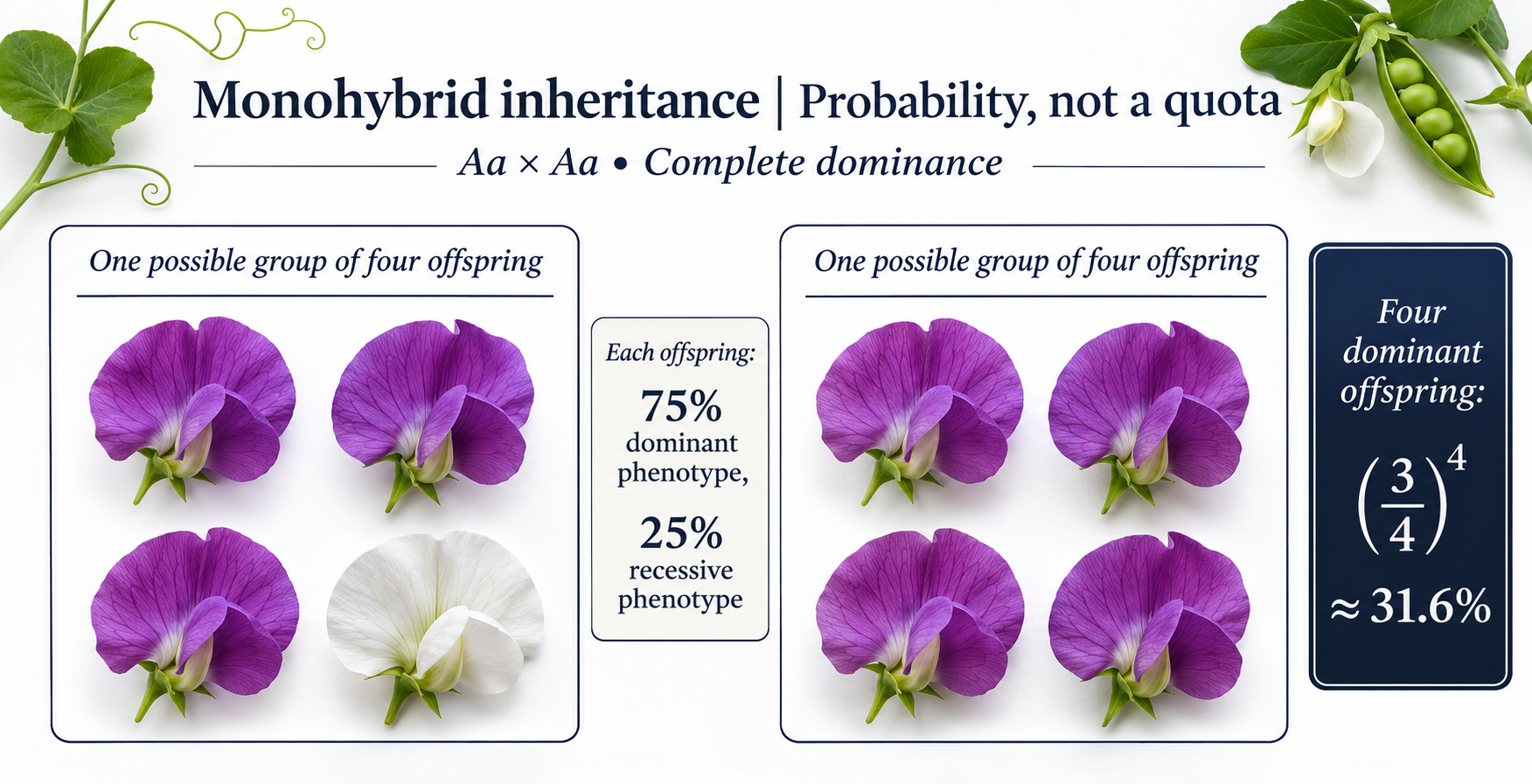
Expected genotype and phenotype probabilities under complete dominance.


Probability, not a quota
Possible groups of four offspring show why a 3:1 ratio is not a guaranteed result.
 BIOLOGY · 5 VISUALSNeuronExplore a myelinated neuron, its structure and signal propagation.
The essentials
Dendrites, cell body, axon, myelin and terminals in a shortened neuron illustration.

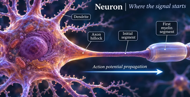
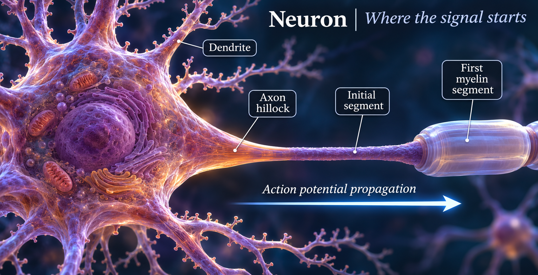
Where the signal starts
The axon hillock and initial segment lead into a myelinated axon.

Insulation with gaps
Schwann-cell myelin surrounds a continuous axon, with nodes between segments.

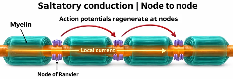
Node to node
Local current spreads beneath myelin and action potentials regenerate at nodes.


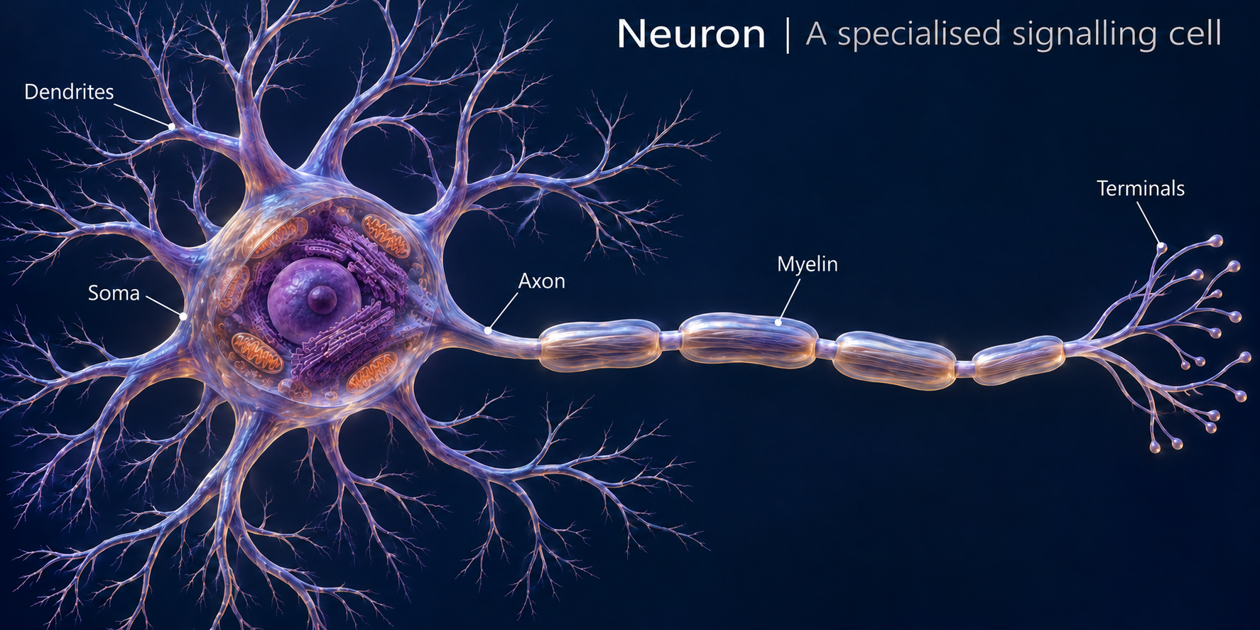
A specialised signalling cell
A detailed illustrative neuron with a shortened axon to show its features together.
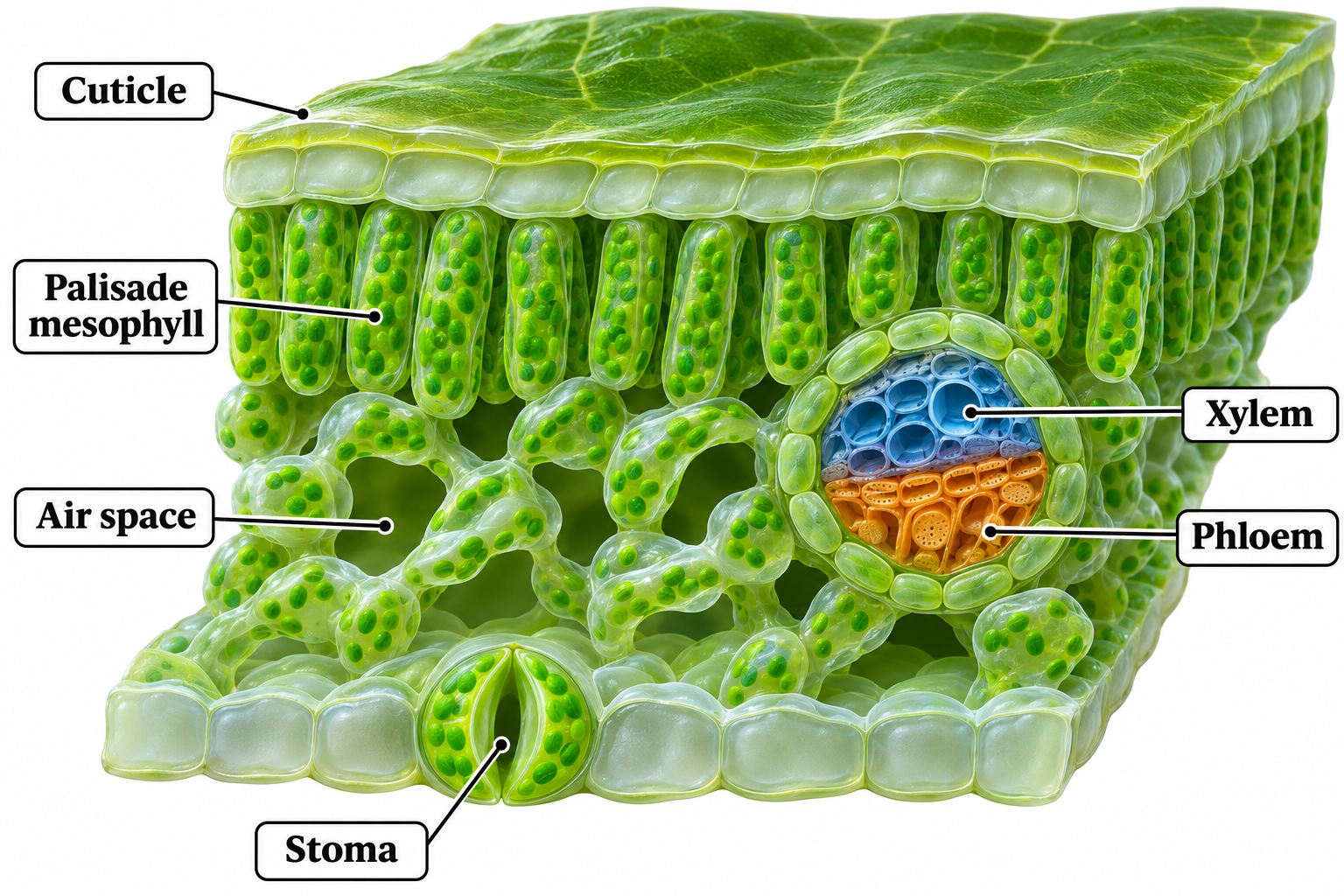
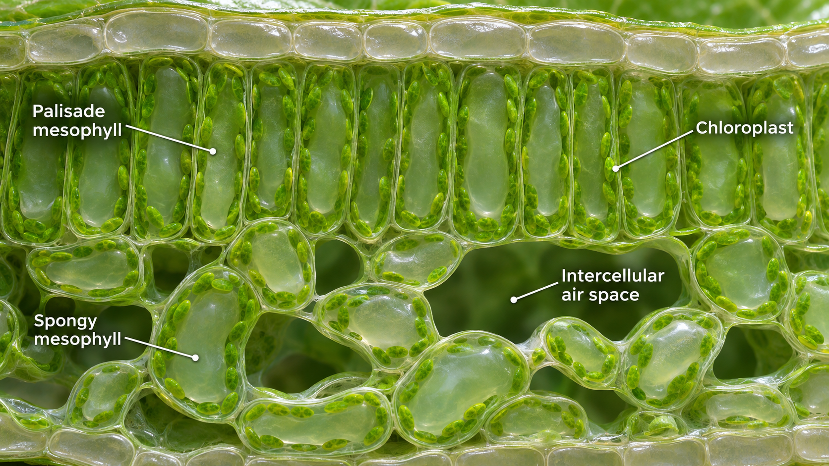
 BIOLOGY · 5 VISUALSLeaf structureExplore the layers, vascular tissues and air spaces of a typical dicot leaf.
The main layers
Upper epidermis, palisade mesophyll, spongy mesophyll and lower epidermis.

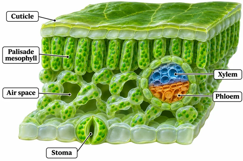
Inside the leaf
A cutaway showing cuticle, air spaces, stoma, xylem and phloem.
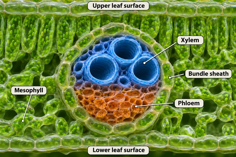
A vascular bundle
Xylem, phloem and bundle sheath within a typical dicot leaf.


Carbon dioxide enters
Follow a route from the stomatal pore through air spaces toward mesophyll cells.

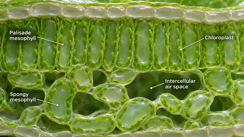
Mesophyll in detail
Palisade and spongy mesophyll, chloroplasts and intercellular air spaces.
 BIOLOGY · 5 VISUALSGuard cellsExplore opening and closure of a typical dicot stomatal pore.
Open and closed
Compare a pair of guard cells around open and closed pores.
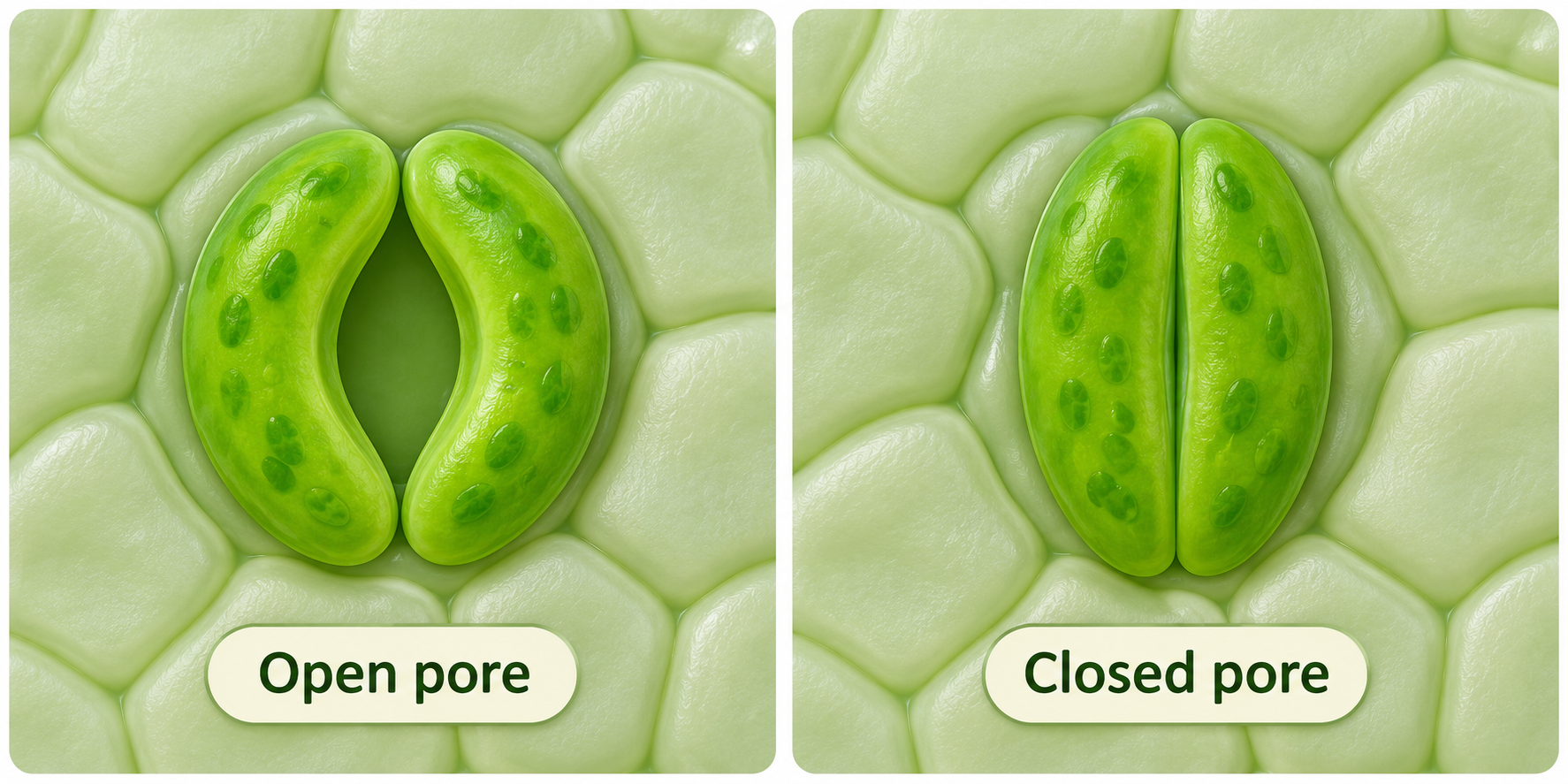

Turgor changes the pore
Higher and lower guard-cell turgor are associated with different pore openings.


Water entry opens the stoma
A simplified sequence of solute accumulation, osmosis and rising turgor.


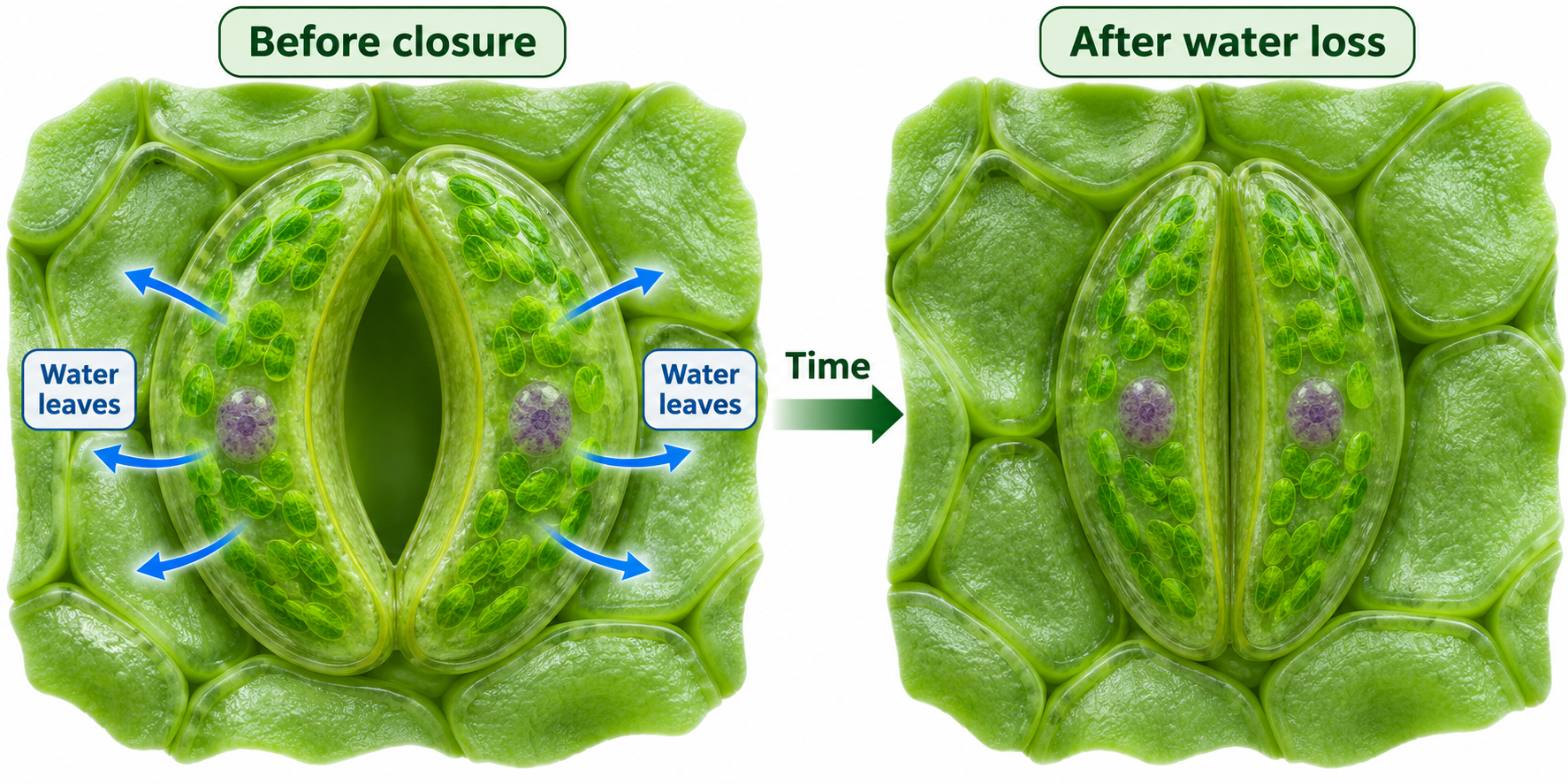
After water loss
Compare guard cells before closure and after water loss.

Inside a guard cell
A detailed illustration of wall thickness, vacuole, chloroplasts and stomatal pore.

 BIOLOGY · 5 VISUALSOxidative phosphorylationFollow electron transport, proton pumping and ATP synthesis across the inner mitochondrial membrane.
The essentials
Electron transport builds a proton gradient that drives ATP synthesis, with oxygen as the final electron acceptor.

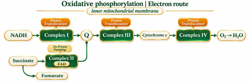
The electron route
NADH and succinate feed electrons into the respiratory chain through different entry points.


Proton pumping
Complexes I, III and IV translocate 4, 4 and 2 protons per pair of electrons from NADH.


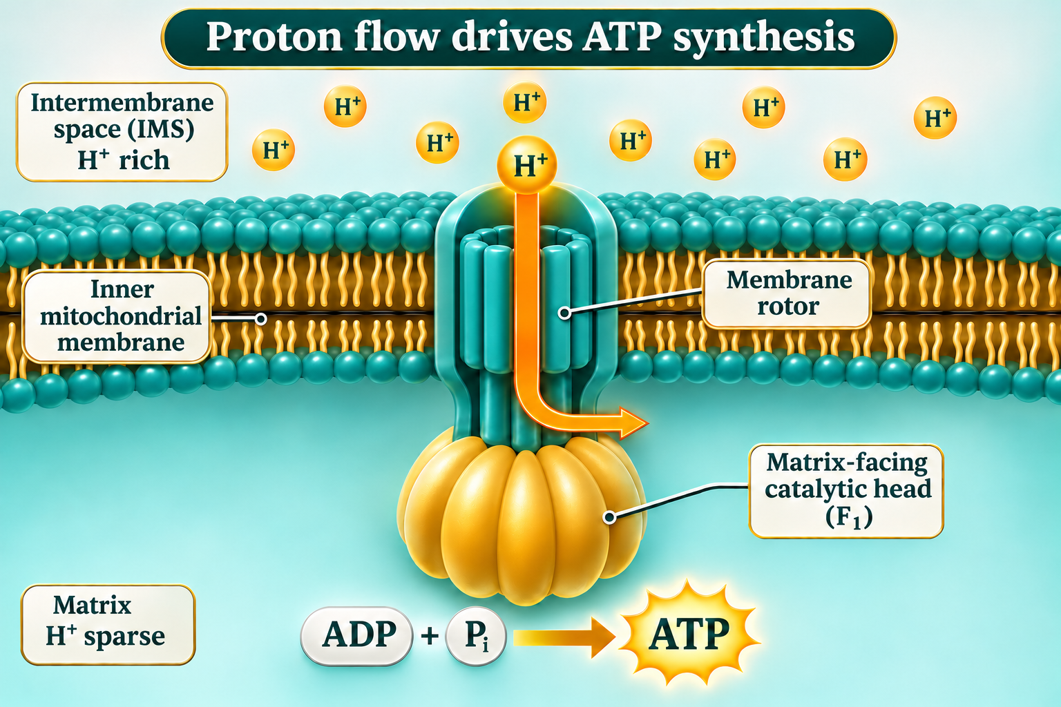
ATP synthase
Protons return to the matrix through ATP synthase, coupling proton flow to ATP production.

Blocking ATP synthase
A coupled mitochondrion with blocked ATP synthase builds a proton gradient while electron transport slows.

 BIOLOGY · 5 VISUALSDNA versus RNACompare strand structure, nucleotide components and the chemical differences between DNA and RNA.
Typical strand structure
DNA is usually double-stranded, while RNA is usually single-stranded and can fold into paired regions.


Shared building blocks
DNA and RNA nucleotides each contain a phosphate, a sugar and a nitrogenous base.

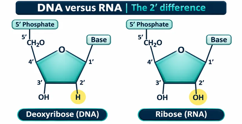
The 2′ difference
Deoxyribose has hydrogen at the 2′ position, where ribose has a hydroxyl group.


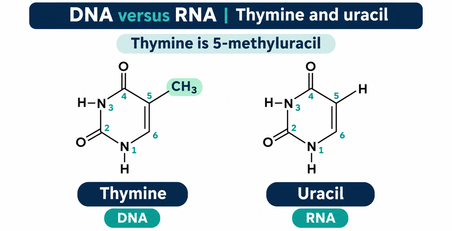
Thymine and uracil
Chemical structures show the methyl group that distinguishes thymine from uracil.
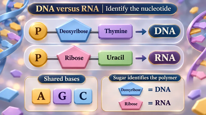
Identify the nucleotide
Sugar and base components help distinguish DNA nucleotides from RNA nucleotides.
 BIOLOGY · 5 VISUALSTest crossesUse recessive offspring and sample size to reason about an unknown genotype under complete dominance.
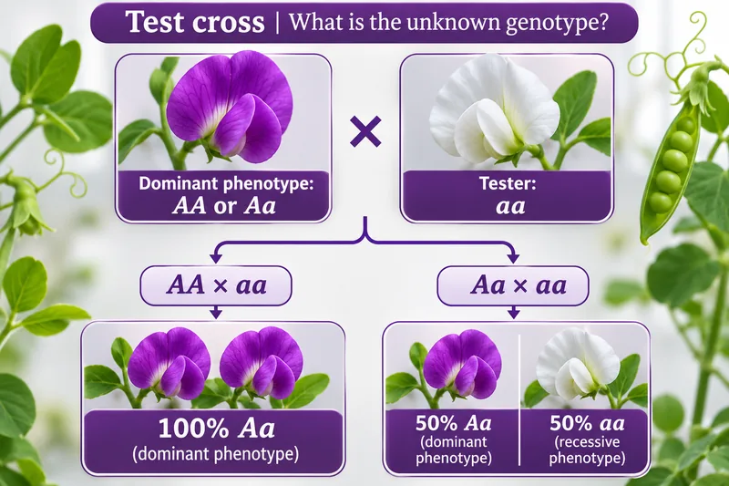
The unknown genotype
Crossing a dominant-phenotype parent with an aa tester distinguishes possible AA and Aa parents.


Compare the possibilities
Punnett squares compare the expected offspring of AA × aa and Aa × aa.


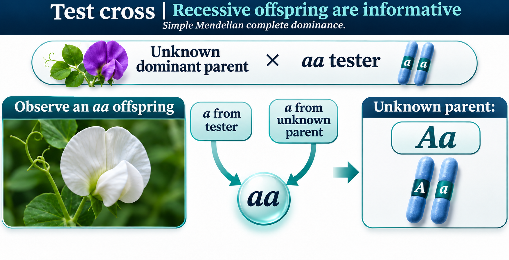
Recessive offspring reveal an allele
An aa offspring demonstrates that the unknown dominant-phenotype parent contributed a recessive allele.

A small sample is not proof
Four dominant offspring still have a 6.25% chance in an Aa × aa cross.


Evidence and sample size
The probability of all-dominant offspring from Aa × aa falls as the number of offspring increases.

 BIOLOGY · 5 VISUALSABO blood-group inheritanceExplore codominance, blood-group genotypes and worked ABO crosses.
Three alleles, four blood groups
A and B antigens distinguish the four ABO blood groups; the A and B alleles are codominant.


Genotype and blood group
A table links the six common ABO genotypes with blood groups and red-cell antigens.


AB × O
A Punnett square gives a 50% probability of group A and 50% of group B for each child.

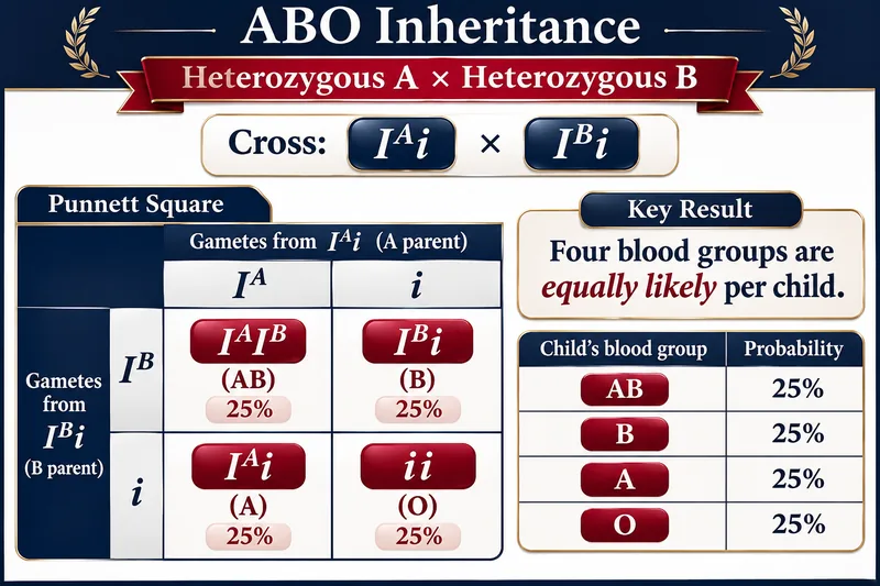
Heterozygous A × heterozygous B
The illustrated cross gives an equal probability of each of the four ABO blood groups.


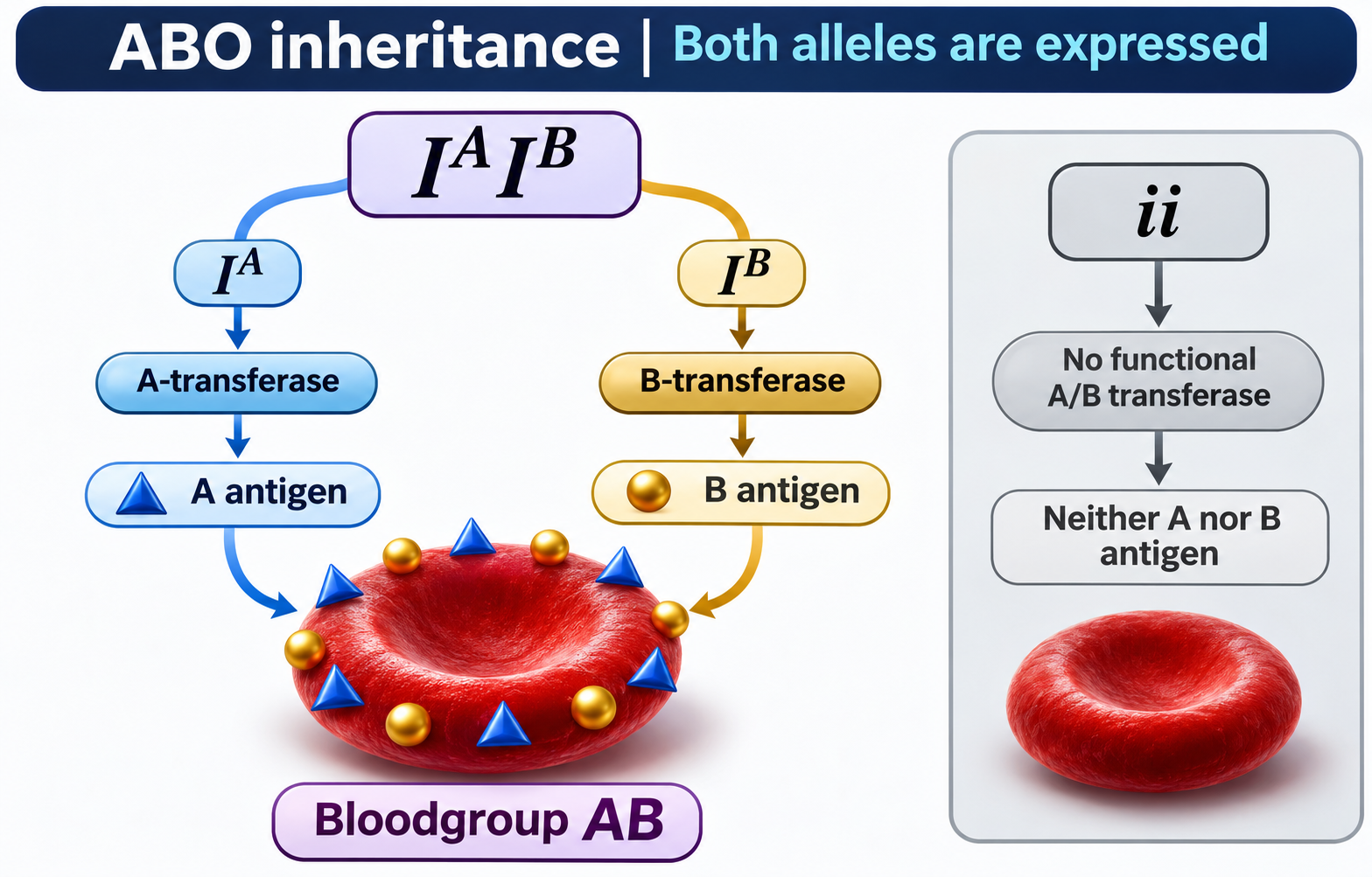
Both alleles are expressed
A and B transferases produce their respective antigens in group AB, unlike the common ii genotype.
 BIOLOGY · 5 VISUALSPCRExplain the PCR cycle, primers, reaction components and idealised amplification.
Three repeating steps
Denaturation, annealing and extension repeat to amplify DNA, with example temperatures shown.


Primers face the target
Opposing primers orient DNA synthesis 5′ to 3′ toward the target region.

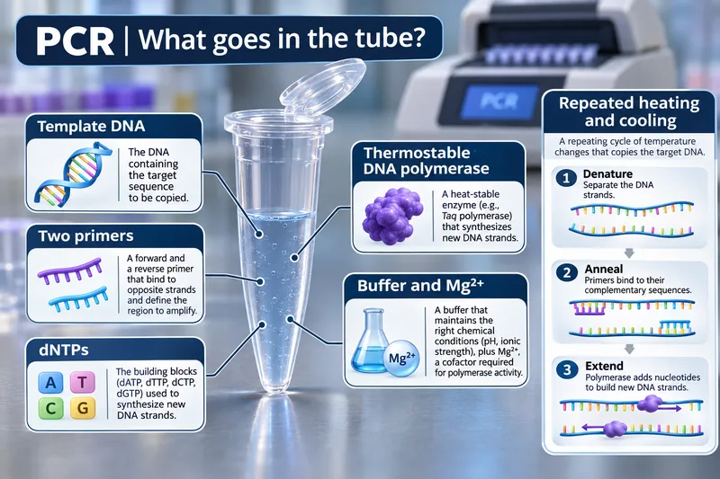
What goes in the tube?
Template DNA, two primers, nucleotides, thermostable polymerase and buffered magnesium support PCR.


Ideal doubling
An ideal 100%-efficiency model doubles the total number of double-stranded DNA molecules each cycle.

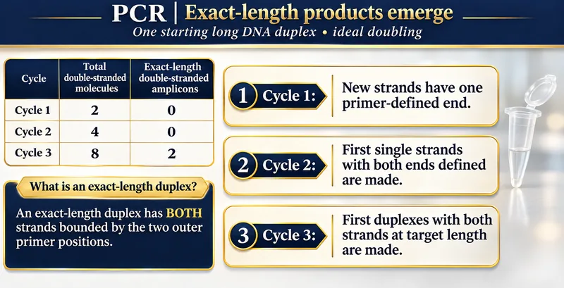
Exact-length products emerge
Starting with a long DNA duplex, exact-length double-stranded amplicons first appear in cycle three.

 BIOLOGY · 5 VISUALSGel electrophoresisFollow DNA migration and interpret bands using illustrative ladders and worked examples.
DNA moves toward positive
Negatively charged DNA migrates toward the positive electrode; smaller fragments travel farther.


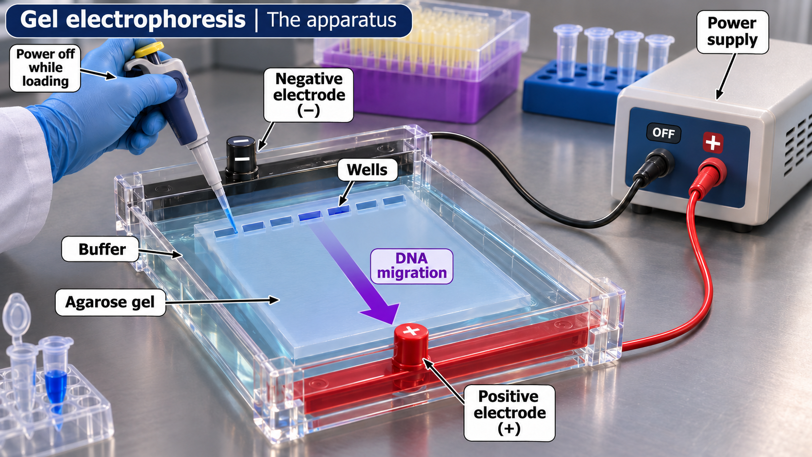
The apparatus
A labelled agarose-gel setup shows wells, buffer, electrodes and the direction of DNA migration.
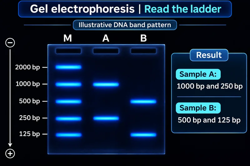
Read the ladder
An illustrative band pattern compares sample fragments with a labelled DNA size ladder.
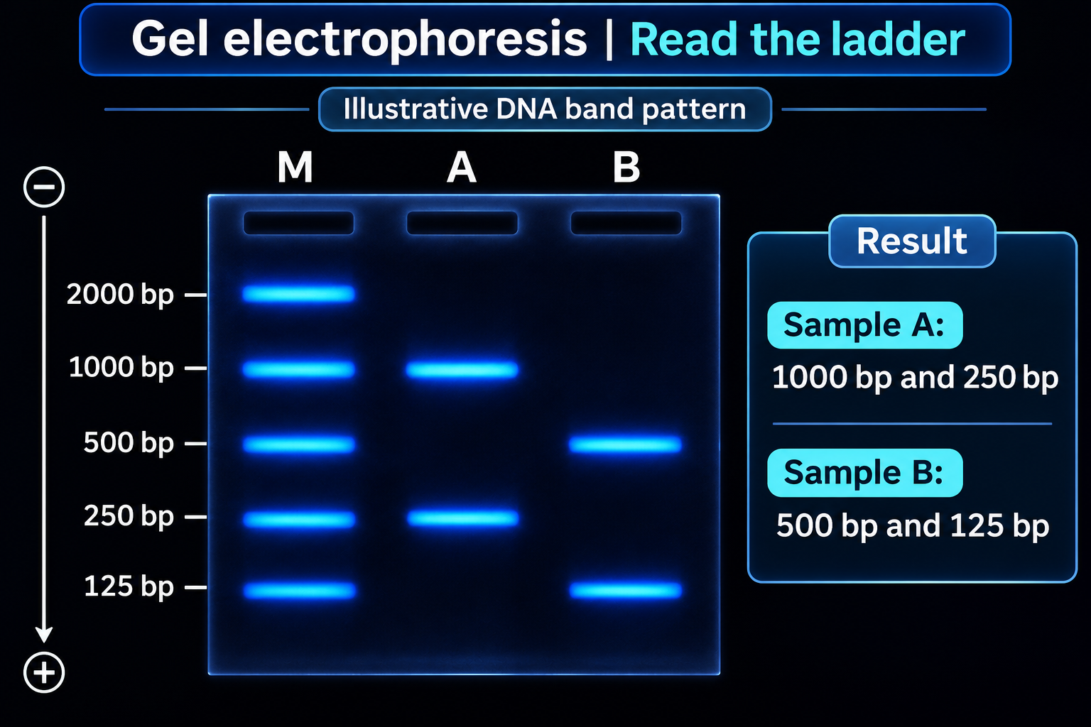

Estimate fragment size
An illustrative semilog calibration estimates a 25 mm band at approximately 707 base pairs.


Same size, different sequence
Equal migration can suggest similar fragment length without establishing identical DNA sequences.

 BIOLOGY · 5 VISUALSNatural selectionConnect inherited variation and reproductive success with population change.
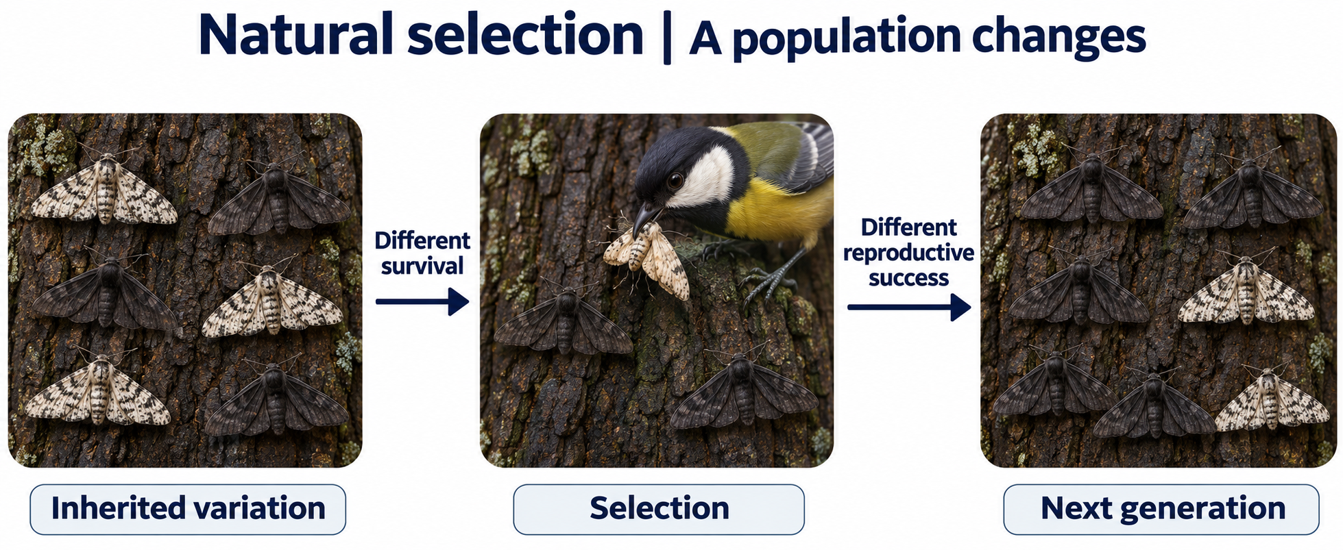
A population changes
A moth example links inherited colour variation, predation and the next generation.
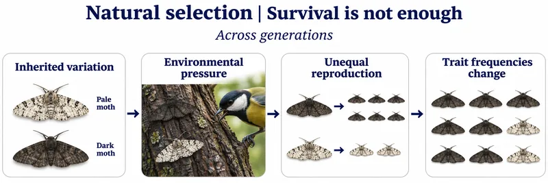
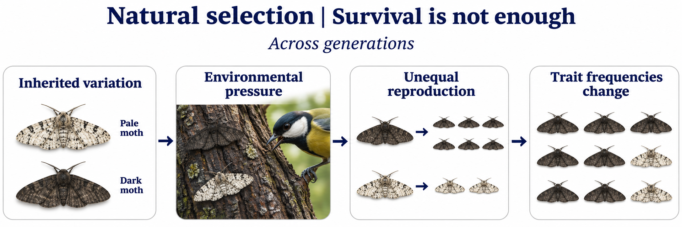
Survival is not enough
Unequal reproductive success changes inherited trait frequencies across generations.
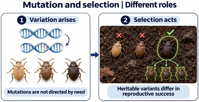
Mutation and selection
Mutations generate variation without being directed by need; selection acts on heritable differences.


When the environment changes
A change in bark colour changes which moth camouflage is favoured by predation.

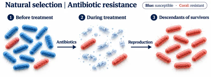
Antibiotic resistance
Resistant bacteria survive treatment and reproduce in this simplified population example.

 BIOLOGY · 5 VISUALSThe heartExplore chambers, valves, pressure-driven flow and the complete circulatory route.
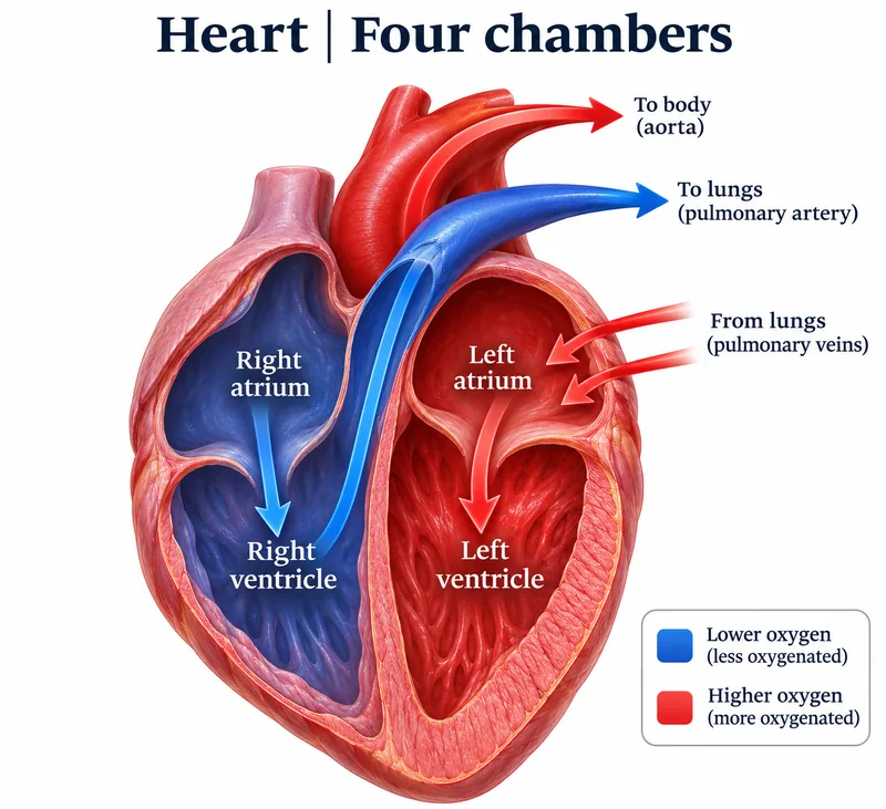
Four chambers
A heart cutaway follows blood through the right and left chambers to the lungs and body.
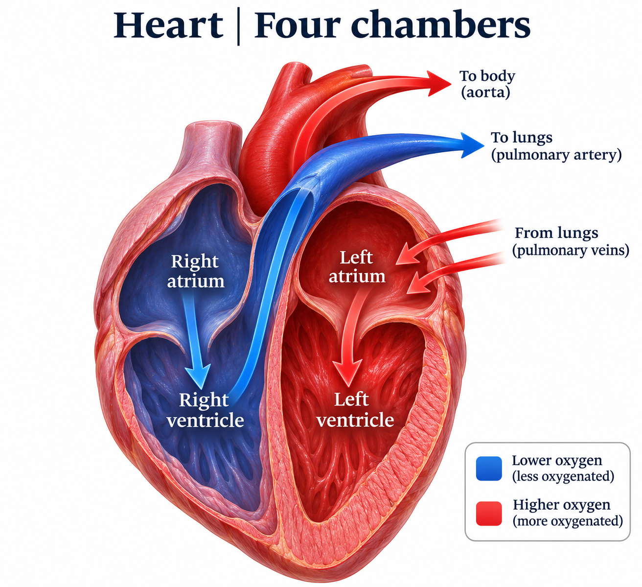

Internal anatomy
A labelled cutaway identifies chambers, septum and major vessels.


Valves guide the flow
Open-valve views compare pulmonary, aortic, tricuspid and mitral valve structures.

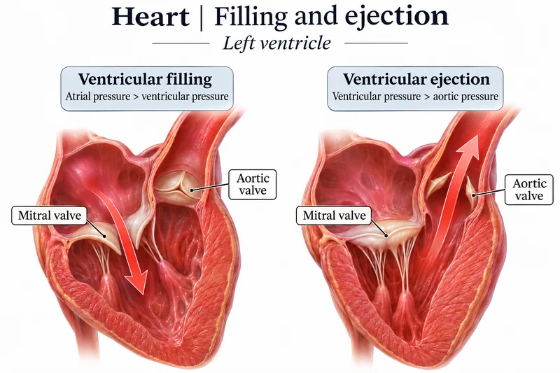
Filling and ejection
Left-ventricular views compare valve positions during filling and ejection.

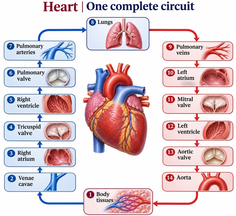
One complete circuit
A numbered route follows blood through the heart, lungs and body tissues.

 BIOLOGY · 5 VISUALSAlveolar gas exchangeRelate the alveolar exchange barrier and partial-pressure gradients to diffusion.
Gas exchange
Oxygen moves from alveolar air into blood while carbon dioxide moves in the opposite direction.

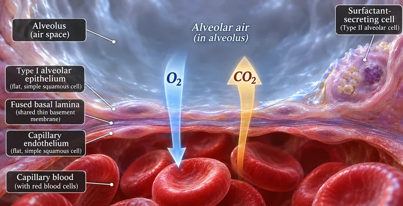
The exchange barrier
A close-up identifies alveolar epithelium, fused basal lamina and capillary endothelium.


Partial-pressure gradients
Typical resting sea-level values illustrate the gradients for oxygen and carbon dioxide exchange.


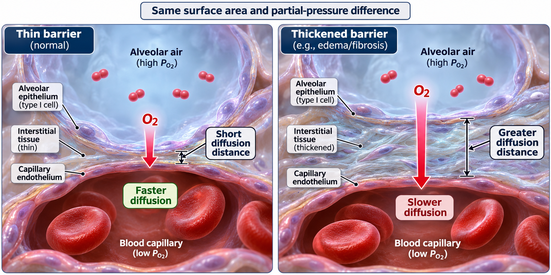
Barrier thickness
With surface area and pressure difference held constant, a thicker barrier slows diffusion.
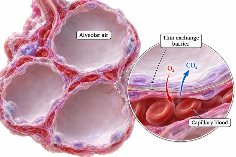
Alveolar tissue
A tissue cutaway and enlarged inset connect alveolar air spaces with the thin blood–air barrier.

 BIOLOGY · 5 VISUALSThe nephronFollow filtrate and explore filtration, the loop of Henle and selective reabsorption.
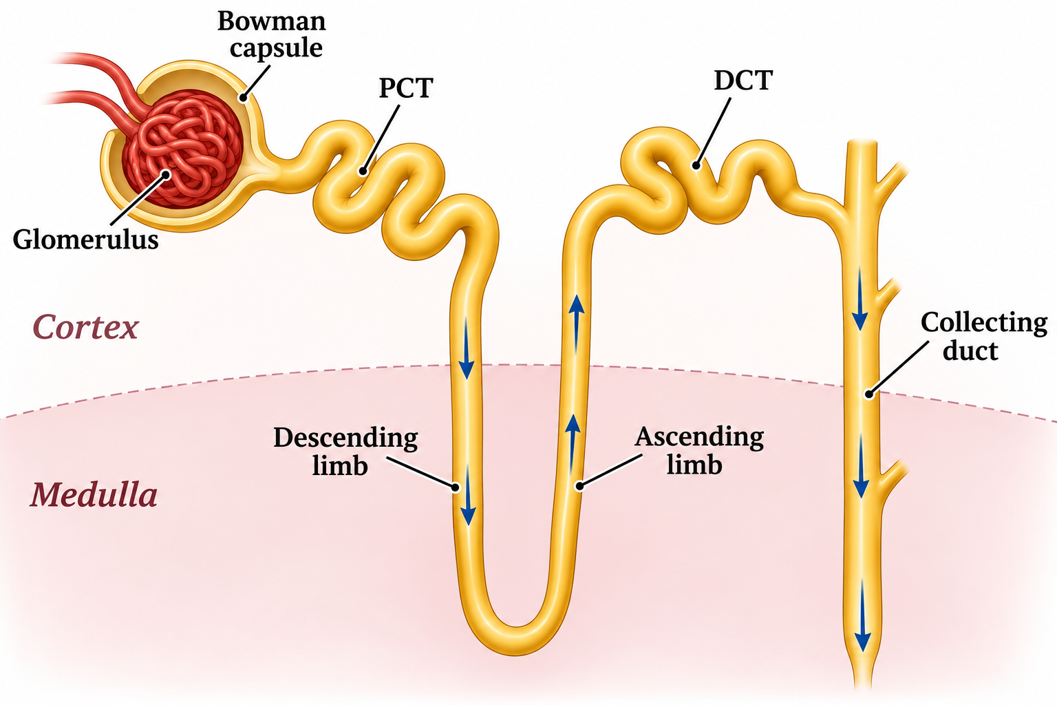
The filtrate route
A labelled nephron traces filtrate through the cortex and medulla into the collecting duct.
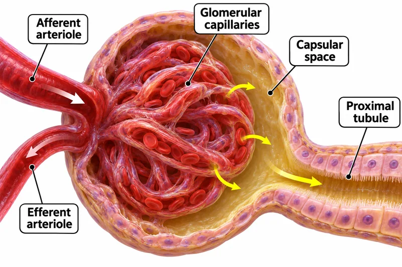
The renal corpuscle
A cutaway shows glomerular capillaries, arterioles, capsular space and the proximal tubule.
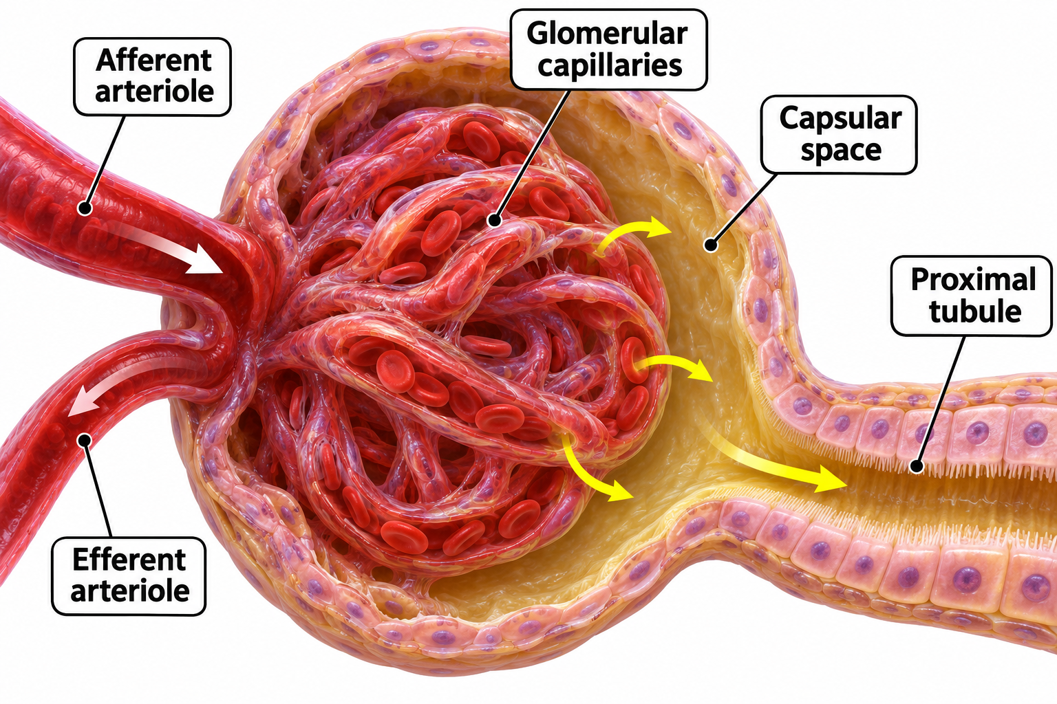

The countercurrent loop
Descending and ascending limbs differ in water permeability and salt transport.

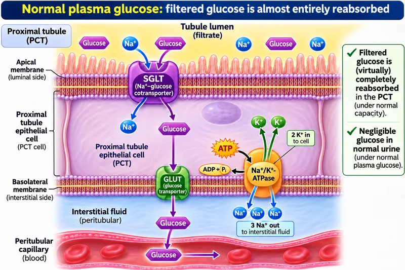
Glucose reabsorption
Proximal-tubule transport links sodium–glucose cotransport, GLUT transport and the sodium–potassium pump.


Filtration is only the start
A comparison follows water, glucose, urea and red blood cells in a healthy kidney.

 BIOLOGY · 5 VISUALSAction potentialsConnect voltage changes with ion channels, firing frequency and propagation.
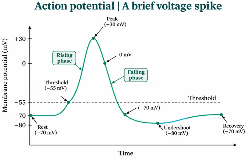
A brief voltage spike
A representative action-potential curve marks threshold, depolarisation, repolarisation and undershoot.


Ion flow changes voltage
Channel states and ion movements are compared during depolarisation, repolarisation and after-hyperpolarisation.

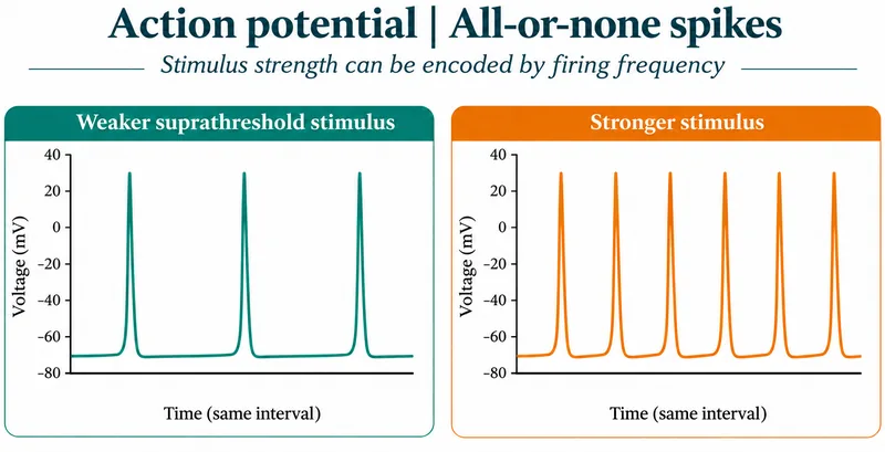
All-or-none spikes
Illustrative traces show a stronger stimulus encoded by higher firing frequency rather than larger spikes.
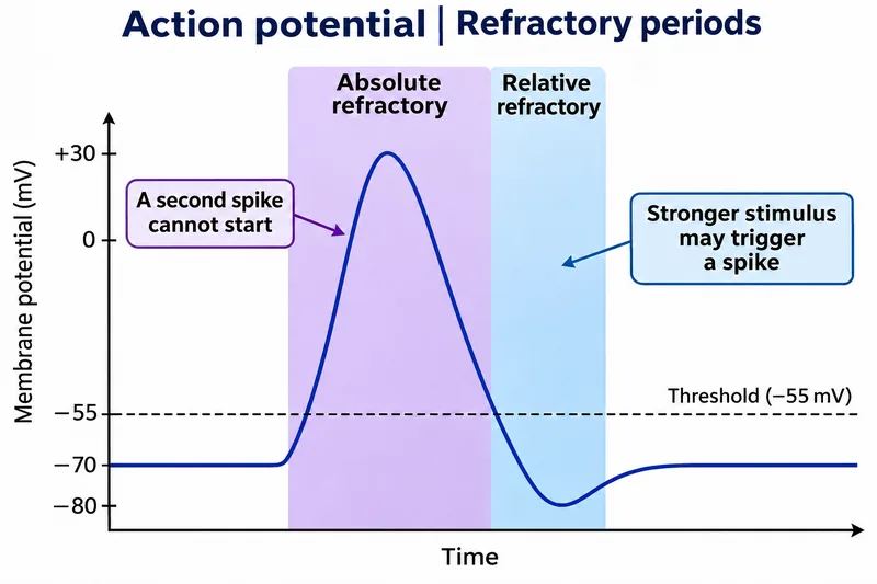
Refractory periods
A representative trace distinguishes absolute and relative refractory periods.

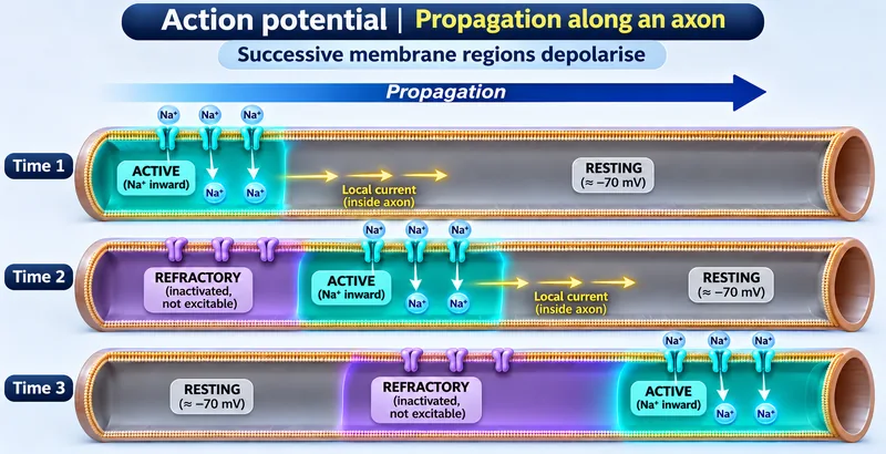
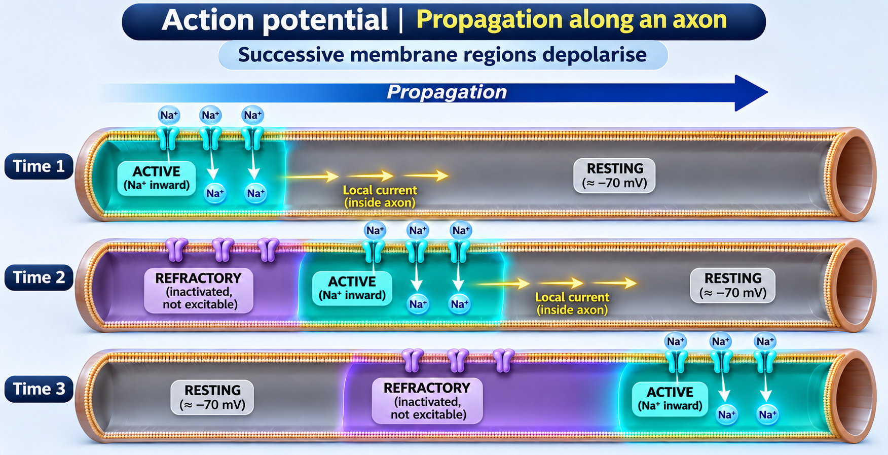
Propagation along an axon
Successive axon regions depolarise as local currents spread and recently active regions become refractory.
 BIOLOGY · 5 VISUALSBlood glucose homeostasisCompare insulin and glucagon responses, glucose transport and glycogen storage.
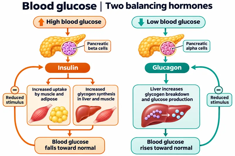
Two balancing hormones
Negative-feedback loops link blood glucose with insulin and glucagon secretion.


After a meal
Insulin supports glucose uptake in muscle and adipose tissue and glycogen synthesis in the liver.


Between meals
Glucagon supports hepatic glucose production through glycogenolysis and gluconeogenesis.

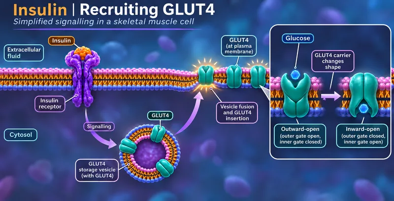
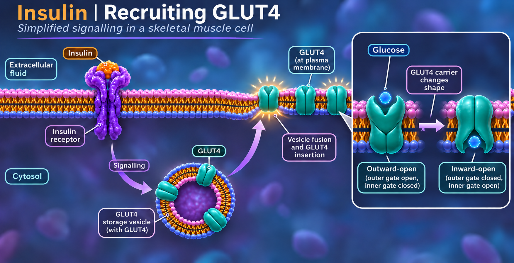
Recruiting GLUT4
A simplified muscle-cell model shows insulin signalling and GLUT4 insertion into the cell membrane.
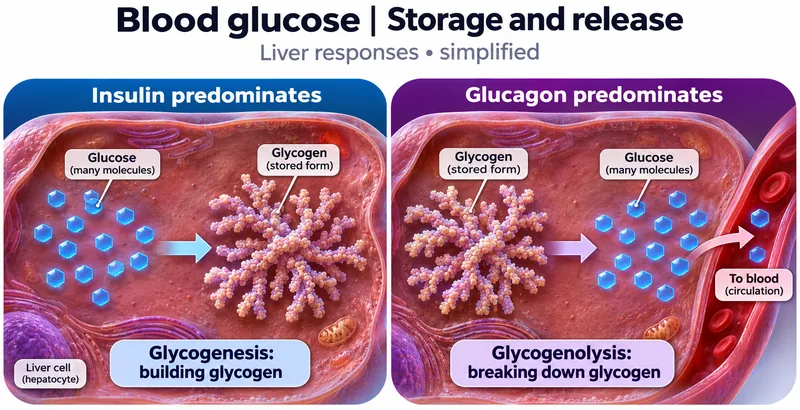
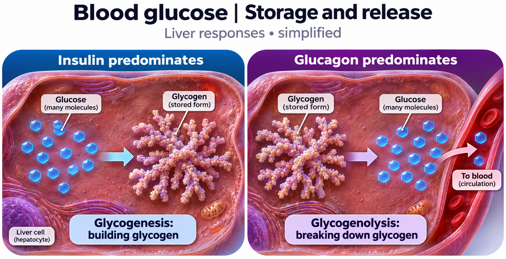
Storage and release
Liver-cell views compare glycogen synthesis and glycogen breakdown.
 BIOLOGY · 5 VISUALSAntibody structureExplore IgG chains and domains, then compare them with deposited antibody structural models.
Two binding sites
An IgG diagram identifies heavy chains, light chains, antigen-binding sites and the Fc region.

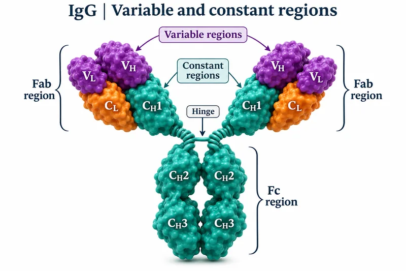
Variable and constant regions
An IgG domain map distinguishes variable regions, constant regions, Fab, Fc and the hinge.


Chains held together
Selected interchain disulfide bonds connect the heavy and light chains of IgG.


IgG2a ribbon model
Protein-only ribbon view of mouse monoclonal antibody Mab231 from PDB 1IGT, with heavy and light chains coloured separately.
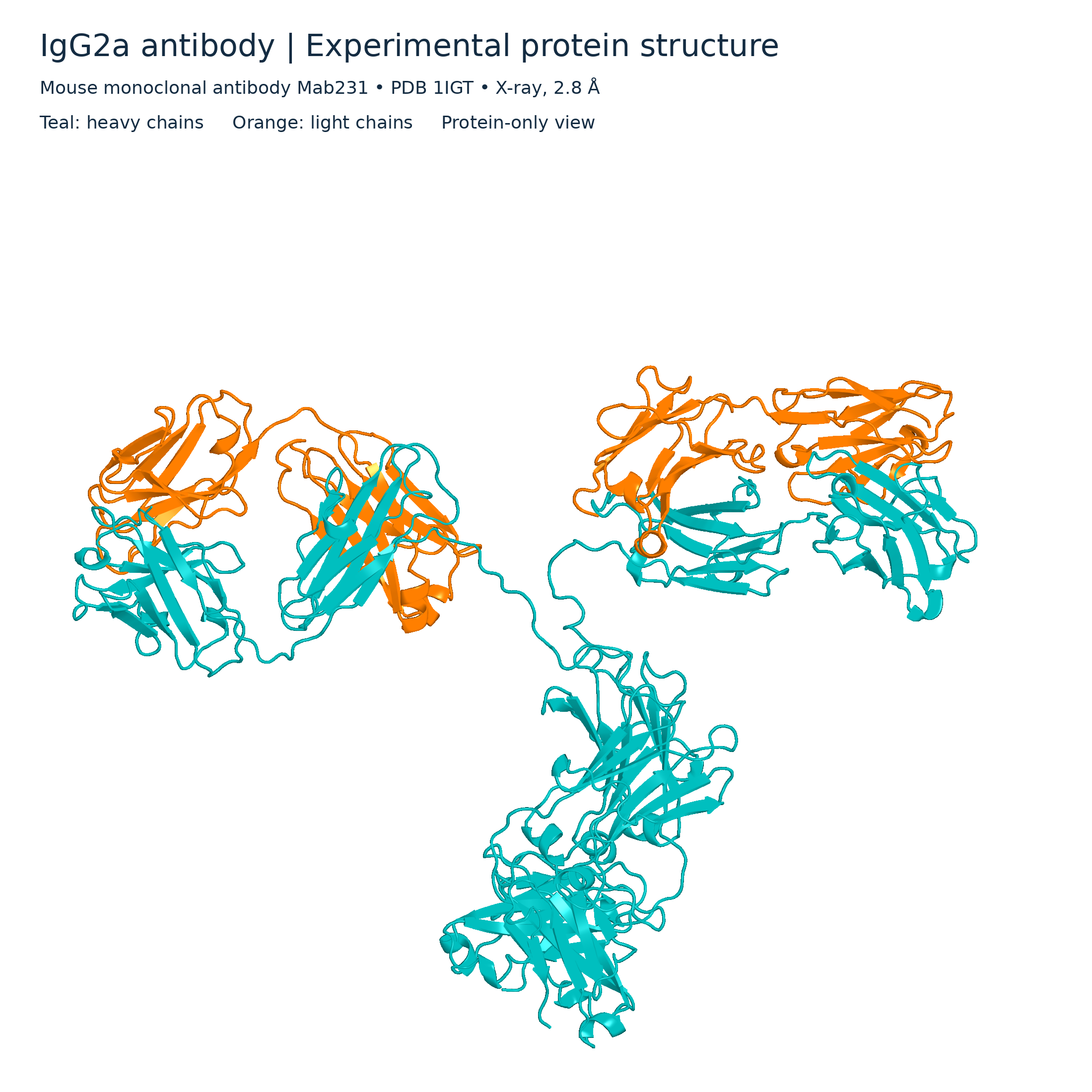

IgG2a molecular surface
Protein-only surface view of the PDB 1IGT antibody structure, with heavy chains in teal and light chains in orange.

 BIOLOGY · 5 VISUALSImmune memoryCompare primary and secondary responses and the role of memory cells.
First and second responses
A qualitative antibody-response curve compares first and repeated exposure to the same antigen.
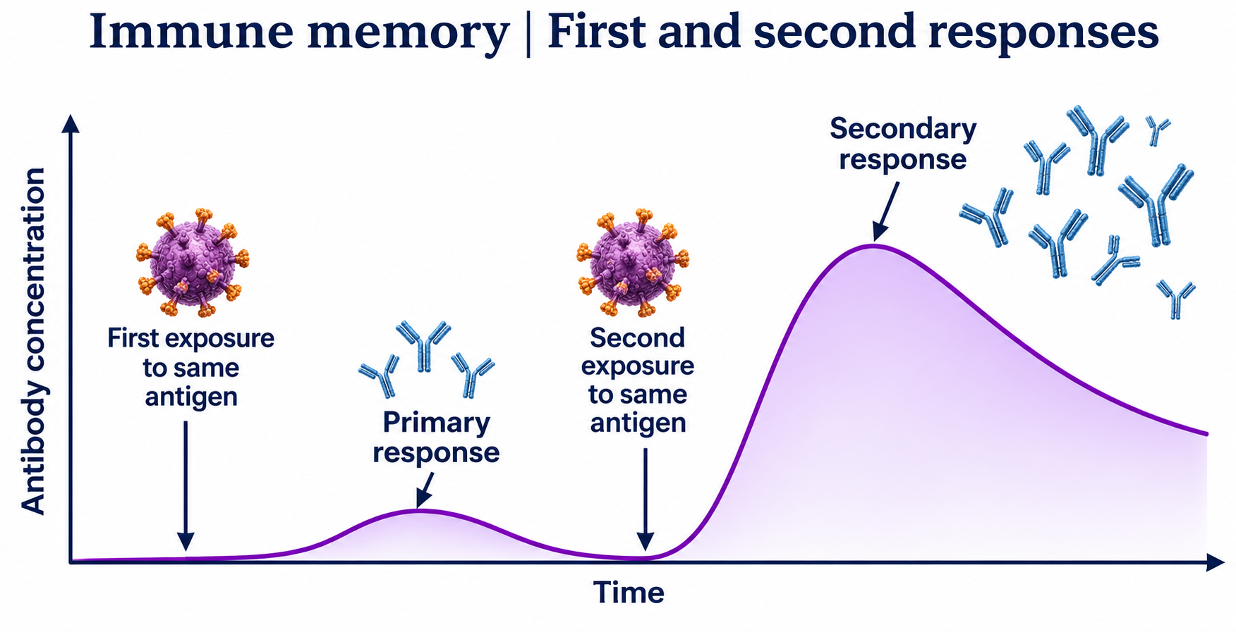

Why the second response is faster
B-cell expansion, plasma cells and memory cells explain a faster response after later exposure.


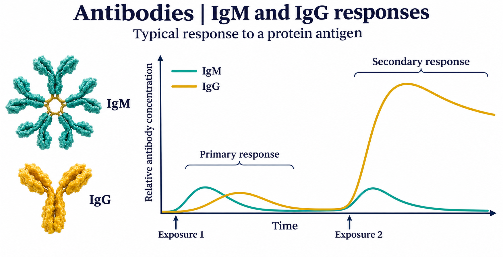
IgM and IgG responses
Qualitative curves compare typical IgM and IgG responses to repeated exposure to a protein antigen.

Vaccination and memory
A simplified adaptive response shows a first vaccine dose, persistent memory cells and a booster.


Specific to the antigen
A qualitative comparison shows memory for antigen A alongside a first response to antigen B.

 BIOLOGY · 5 VISUALSVilli and absorptionConnect intestinal surface area with nutrient transport into blood and lymph.
More surface for absorption
Nested views distinguish intestinal folds, villi and the microvilli on epithelial cells.


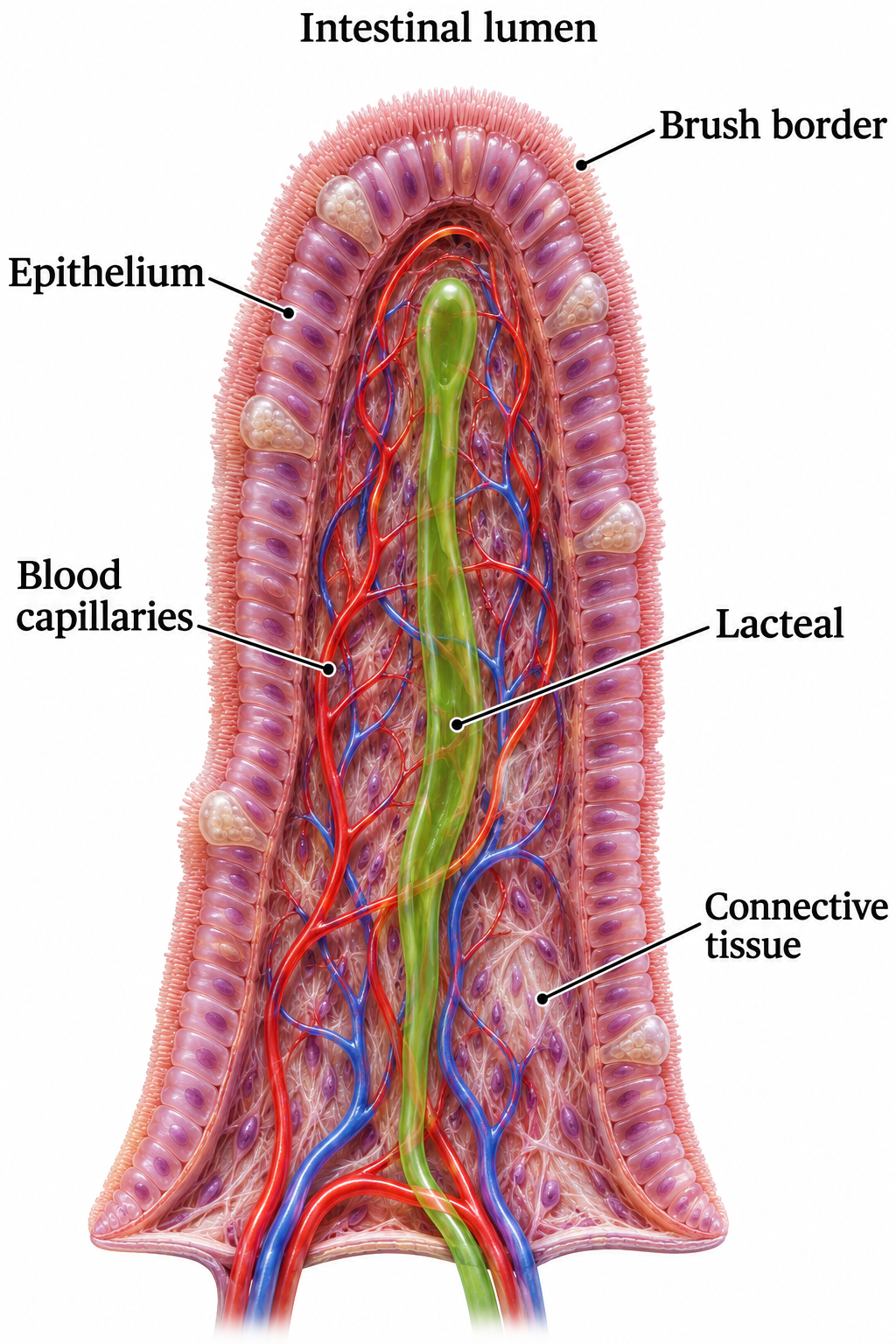
Inside a villus
A villus cutaway identifies epithelium, blood capillaries, lacteal and connective tissue.

Microvilli
A brush-border close-up shows microvilli, actin bundles and the terminal web.


Glucose into the blood
A simplified enterocyte model shows SGLT1, GLUT2 and the sodium–potassium pump supporting glucose absorption.


Long-chain lipids into lymph
Absorbed lipid products are rebuilt and packaged into chylomicrons before entering a lacteal.

 BIOLOGY · 5 VISUALSProtein digestionFollow dietary proteins from hydrolysis to absorption through intestinal cells.
Chains to building blocks
Endopeptidases and exopeptidases break proteins into smaller peptides and amino acids.


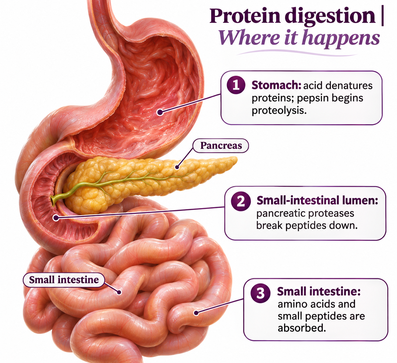
Where digestion happens
A digestive-system view locates protein digestion in the stomach and small intestine.

Activating pancreatic proteases
A simplified pathway shows enteropeptidase activating trypsin and trypsin activating other pancreatic zymogens.


Through the intestinal cell
Simplified transport routes show amino-acid and small-peptide absorption into an enterocyte and onward to blood.

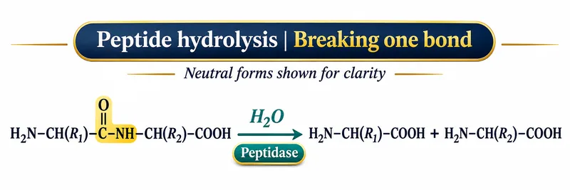
Breaking one peptide bond
A hydrolysis reaction shows water splitting a peptide bond, using neutral chemical forms for clarity.

 BIOLOGY · 5 VISUALSTranspirationTrace water from soil to air and relate transpiration to cohesion, tension and humidity.
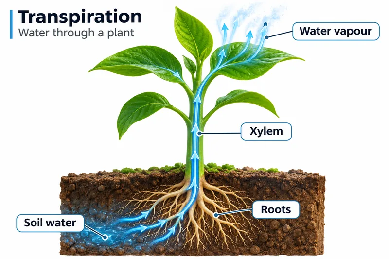
Water through a plant
Water moves from soil through roots and xylem before leaving leaves as water vapour.
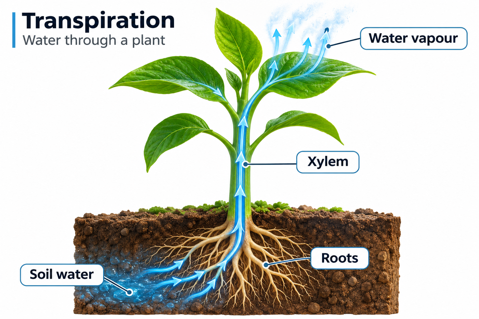

From root to leaf
Enlarged root-hair and xylem views connect water uptake with transport through the plant.


Evaporation then diffusion
Water evaporates from wet mesophyll cell walls and vapour diffuses through stomatal pores.


Cohesion and tension
Evaporation creates tension while cohesion helps maintain a continuous water column in xylem.


Humidity and water loss
At equal temperature, airflow and stomatal opening, drier air produces a steeper water-vapour gradient.

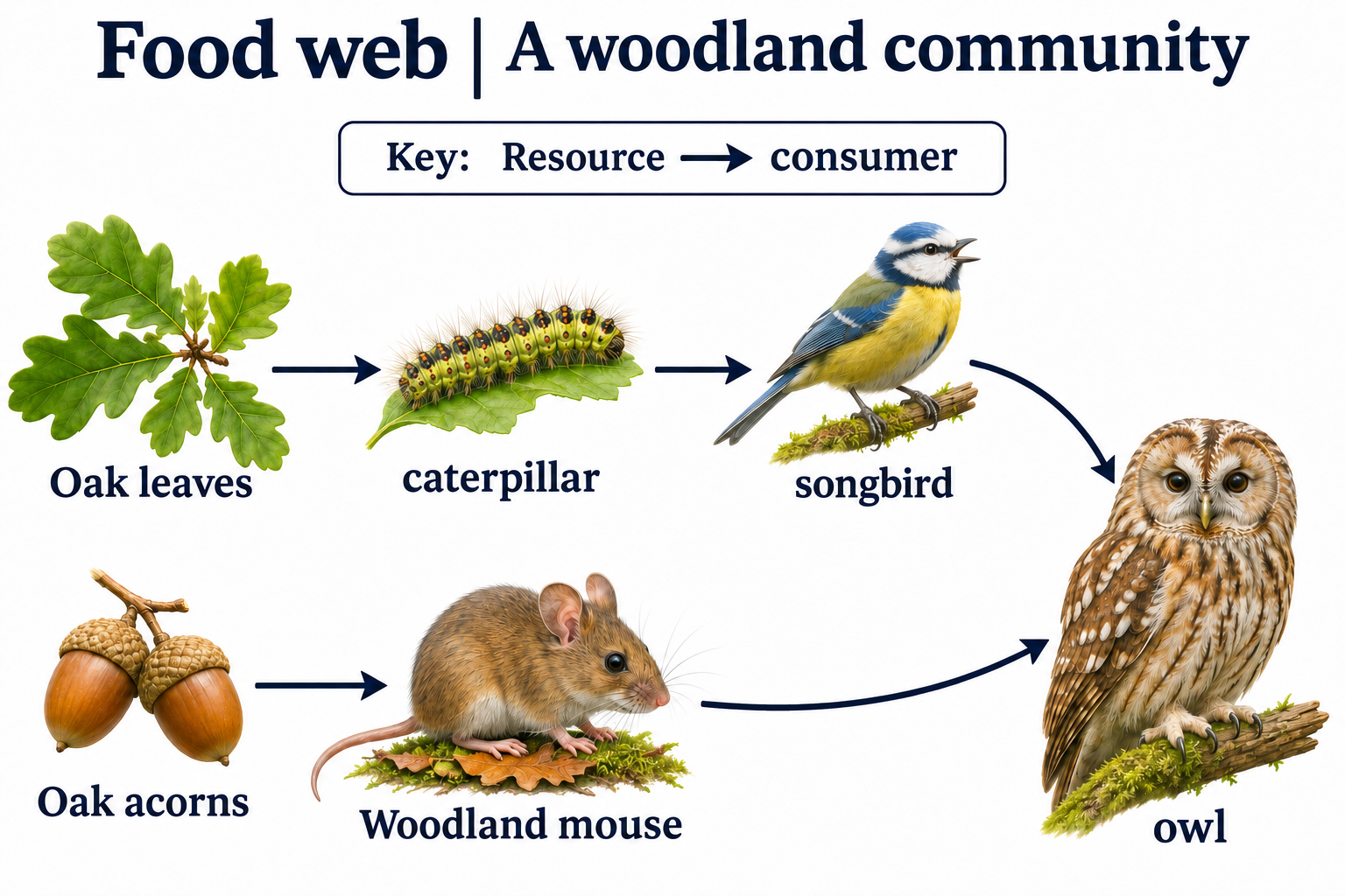
 BIOLOGY · 5 VISUALSFood websRead feeding relationships and explore omnivory, predators and decomposers.
Meadow connections
Arrows run from food to consumer in two connected examples of meadow feeding relationships.


A woodland community
Oak leaves and acorns support consumers and predators in a simplified woodland web.
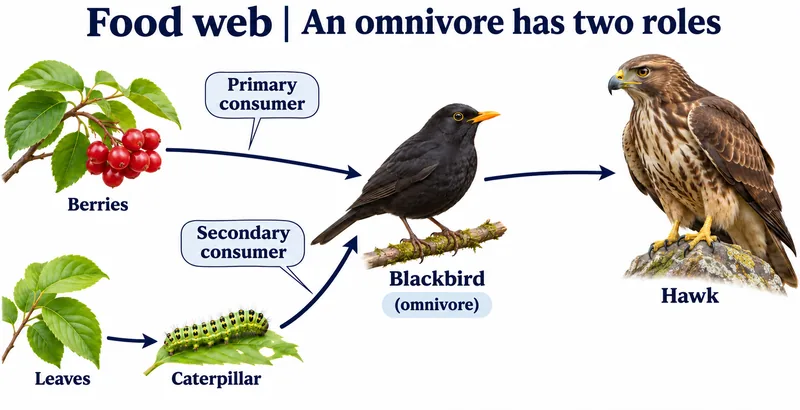
An omnivore has two roles
A blackbird feeding on berries and caterpillars occupies different trophic roles.

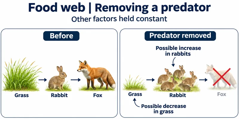
Removing a predator
A simplified example predicts possible rabbit increases and grass decreases after fox removal.


Decomposers receive material
Dead material and waste pass to decomposers, with mineral nutrients returned to plants.

 BIOLOGY · 5 VISUALSEcological pyramidsDistinguish energy, biomass and numbers using diagrams and illustrative calculations.
Less energy at each level
Illustrative energy-flow values decrease across producer and consumer levels.


Three different measures
Energy, biomass and numbers pyramids measure different properties and use different units.


Biomass can invert
Rapid phytoplankton turnover can support an inverted standing-biomass pyramid while energy flow remains upright.


A transfer-efficiency example
Illustrative values give a 10% transfer efficiency from producer to primary consumer.


Numbers and organism size
Grassland and woodland examples show how one large producer can support many consumers.

 BIOLOGY · 5 VISUALSThe carbon cycleFollow carbon through organisms, soils, oceans and long-term stores.
Carbon through living things
Photosynthesis, feeding, decomposition and respiration connect organisms with atmospheric carbon dioxide.
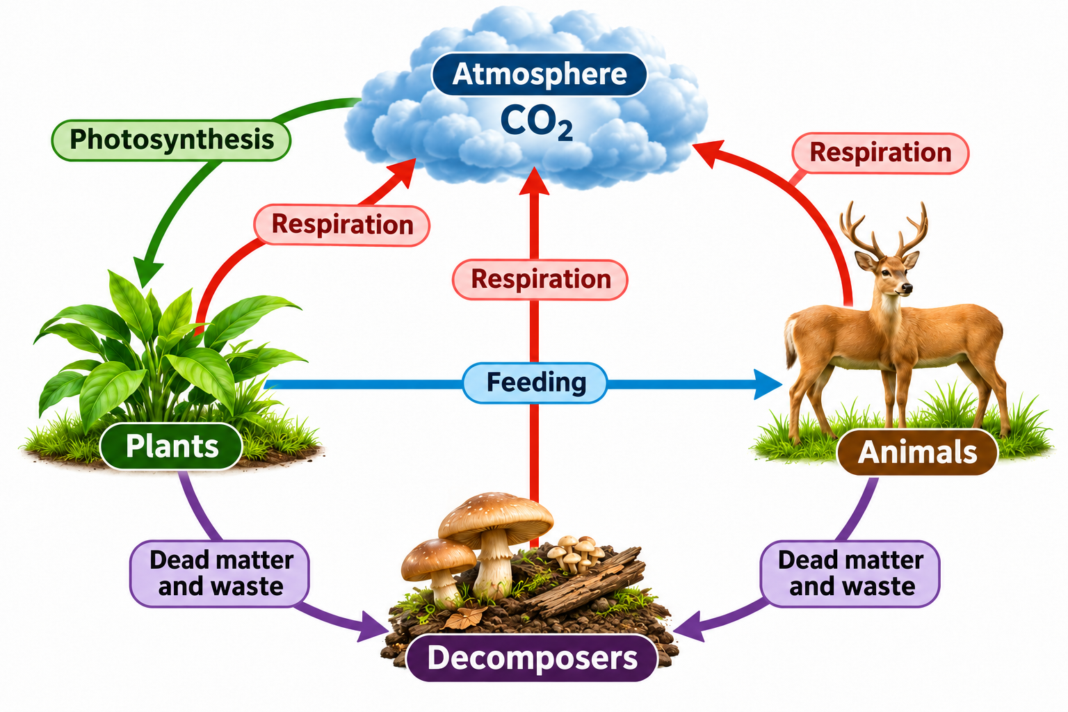

Land and ocean stores
Carbon moves among vegetation, soil, atmosphere and surface and deep ocean stores.


Stored carbon and combustion
Burial and geological transformation store carbon in coal, while combustion releases carbon dioxide.


Fast and slow pathways
Biological cycling is compared with long-term storage and fossil-fuel combustion.
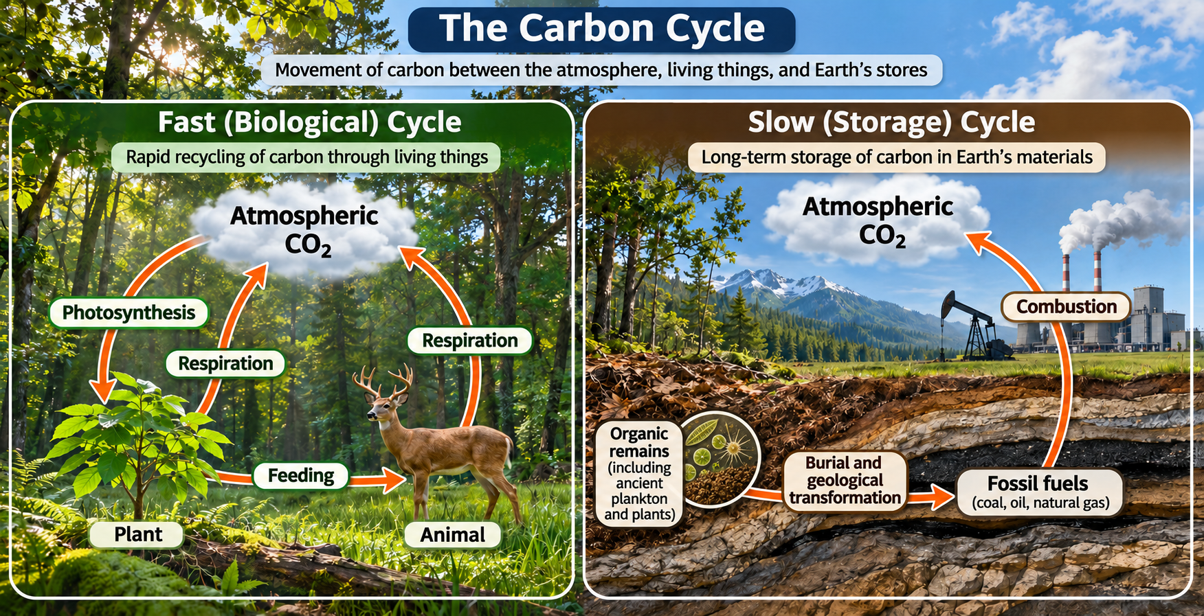

Follow a carbon atom
One possible route takes carbon from atmospheric carbon dioxide through a leaf, herbivore and decomposer.

 BIOLOGY · 5 VISUALSThe nitrogen cycleExplore fixation, soil transformations and nitrogen movement through food chains.
Nitrogen-cycle essentials
Fixation, uptake, feeding, mineralisation and denitrification link major nitrogen stores.


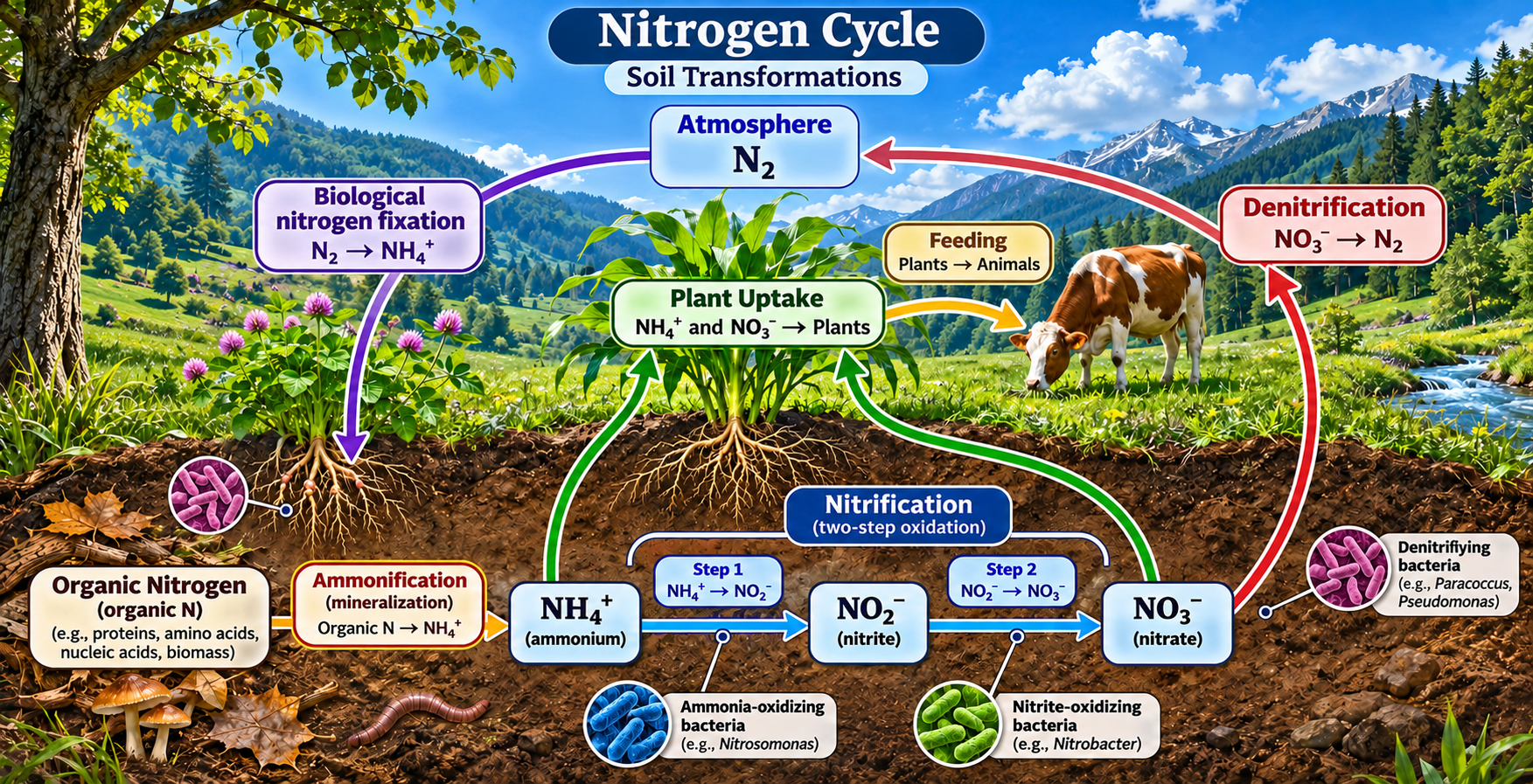
Soil transformations
A detailed soil cycle distinguishes ammonification, nitrification, uptake and denitrification.

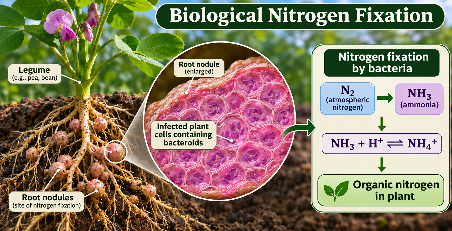
Biological nitrogen fixation
A legume root-nodule view shows bacterial fixation of atmospheric nitrogen and its entry into organic compounds.

Nitrification and denitrification
The comparison distinguishes microbial oxidation in aerobic soil from reduction under low-oxygen conditions.

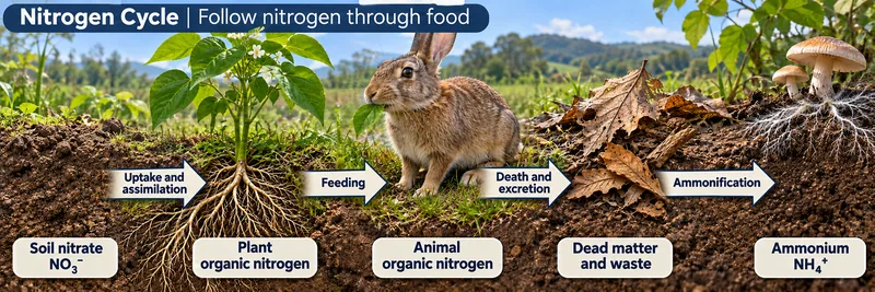
Nitrogen through food
Nitrogen passes from soil nitrate into plants, animals, dead matter and ammonium.

 BIOLOGY · 5 VISUALSPopulation growth and carrying capacityUse idealised population models to explore limiting resources and density dependence.
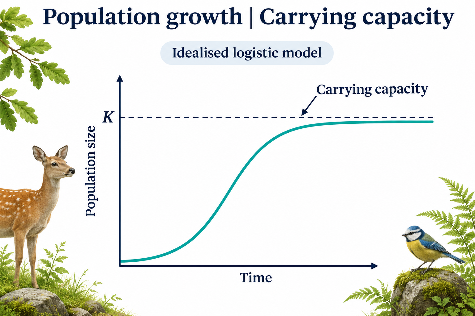
Carrying capacity
An idealised logistic curve approaches carrying capacity K.

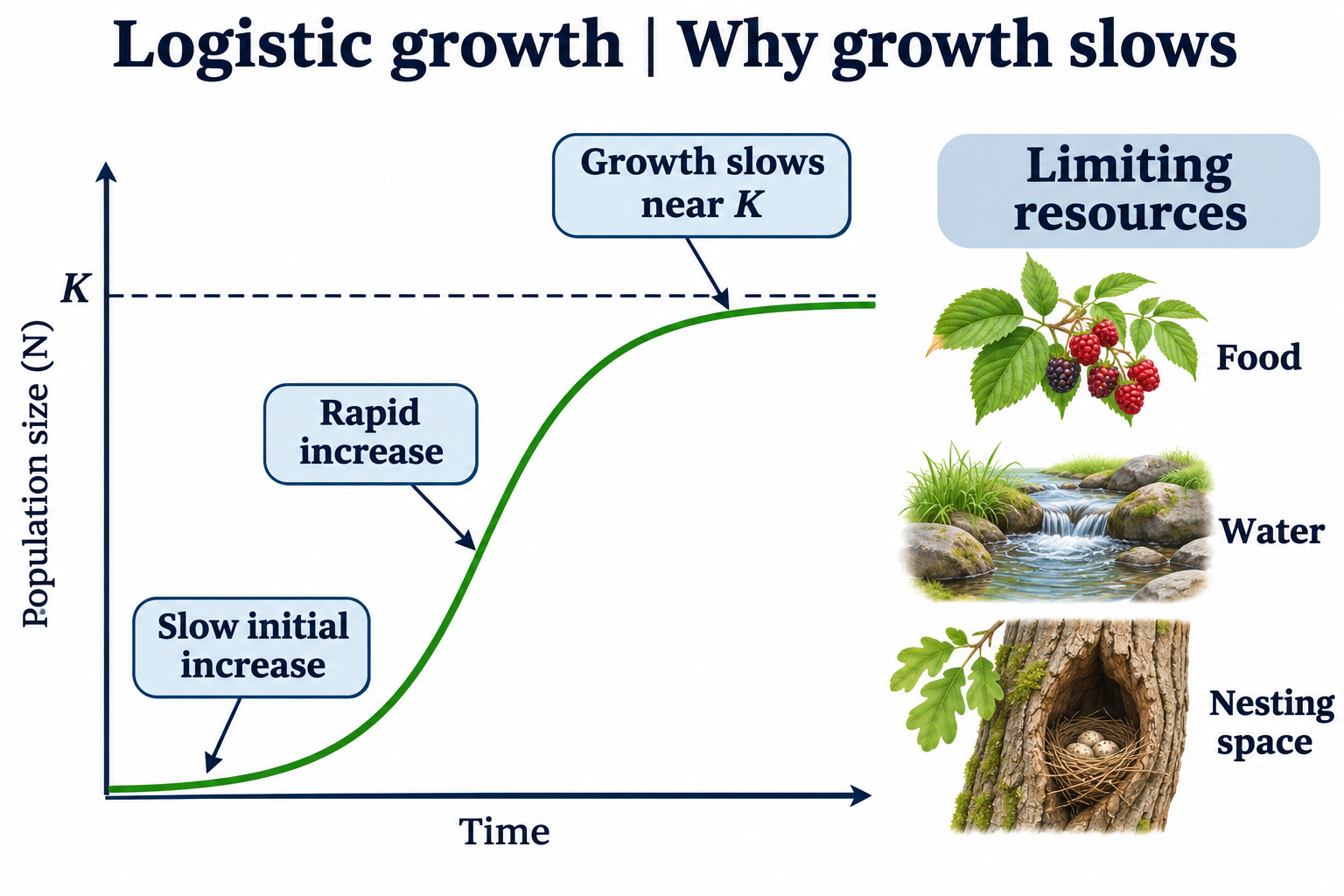
Why growth slows
Food, water and nesting space illustrate resources that can limit population growth.
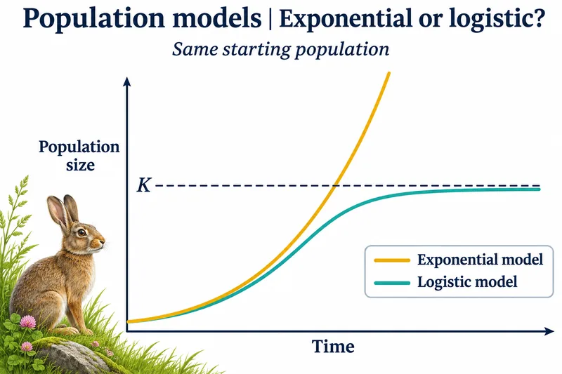
Exponential or logistic?
Idealised curves compare exponential and logistic growth from the same starting population.

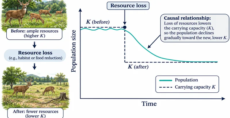
When resources are lost
A conceptual model shows a population declining toward a lower carrying capacity after resource loss.

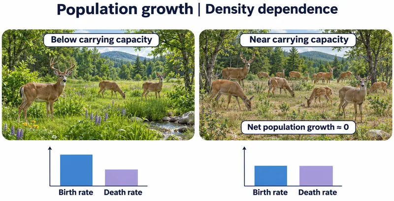
Density dependence
Illustrative birth and death rates are compared below and near carrying capacity.

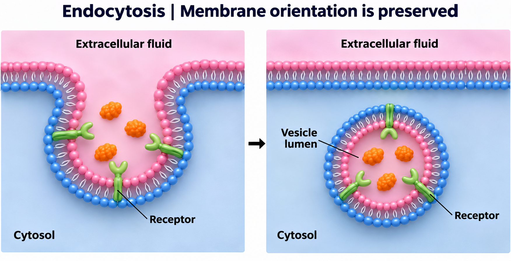
 BIOLOGY · 5 VISUALSEndocytosisExplore vesicle formation, selective uptake and preservation of membrane orientation.
Membrane to vesicle
Three stages show the plasma membrane enclosing extracellular cargo in an internal vesicle.


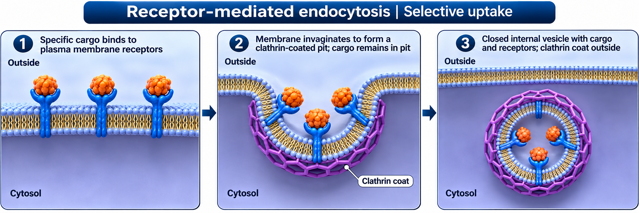
Receptor-mediated uptake
Receptors select cargo as a clathrin-coated pit forms and buds into the cell.

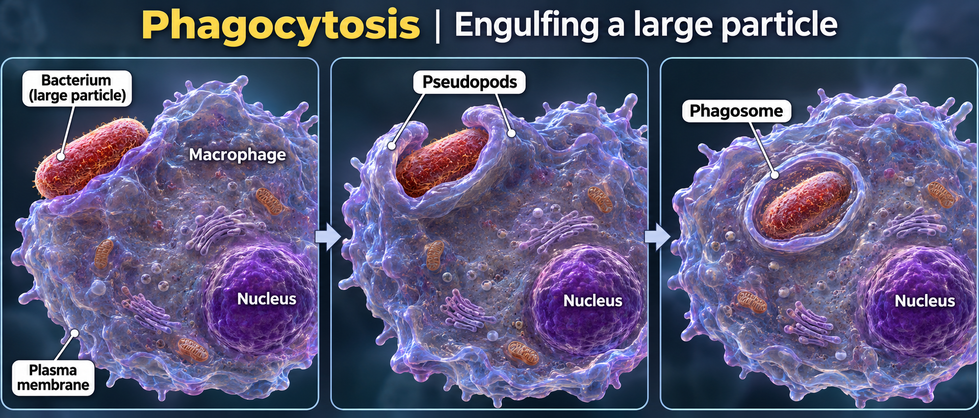
Phagocytosis
A macrophage extends pseudopods around a bacterium and encloses it in a phagosome.

Membrane orientation
The extracellular-facing membrane surface becomes the lumen-facing surface of the vesicle.
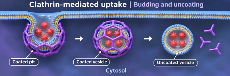
Budding and uncoating
A clathrin-coated pit becomes a coated vesicle and then sheds its coat.

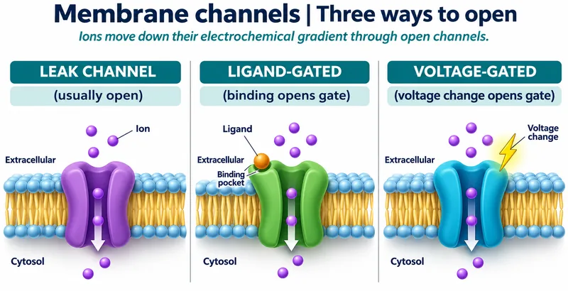 BIOLOGY · 5 VISUALSMembrane channelsCompare channel gating and explore a deposited bacterial potassium-channel structure.
Three ways to open
Leak, ligand-gated and voltage-gated channels allow ions to move down electrochemical gradients.


Ligand-gated opening
A conceptual channel model shows ligand binding changing a closed pore into an open pore.


Sodium-channel states
A conceptual voltage-gated sodium-channel model compares resting, open and inactivated states.

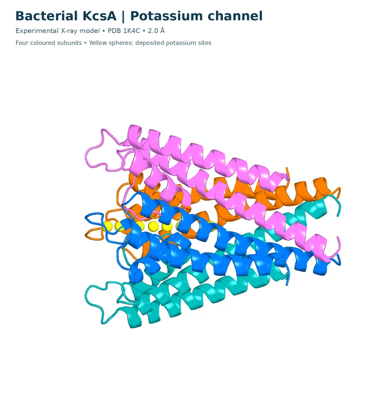
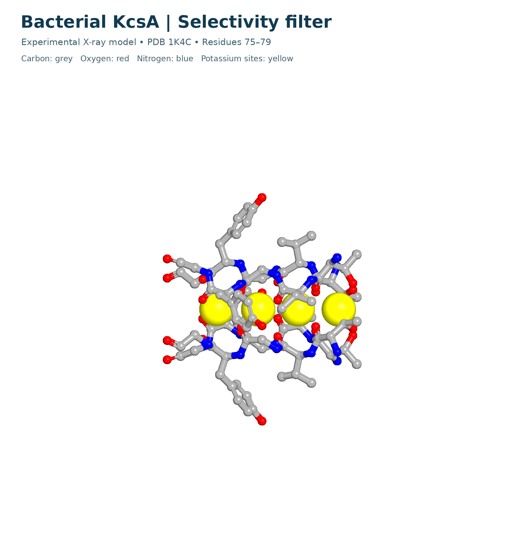
KcsA potassium channel
A ribbon model from PDB 1K4C shows four bacterial KcsA subunits and deposited potassium sites.


KcsA selectivity filter
The PDB 1K4C filter, residues 75–79, is shown with element colours and deposited potassium sites.
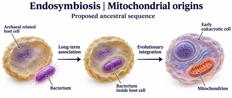 BIOLOGY · 5 VISUALSEndosymbiosisExplore organelle origins, supporting evidence and evolutionary integration.
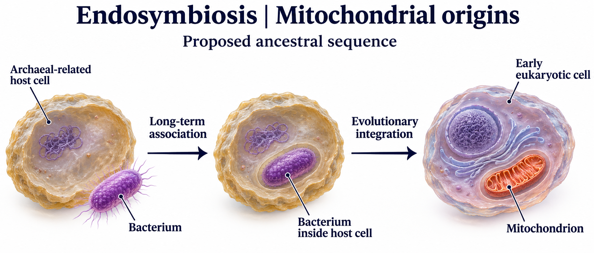
Mitochondrial origins
A proposed ancestral sequence links an archaeal-related host and bacterium with mitochondrial integration.

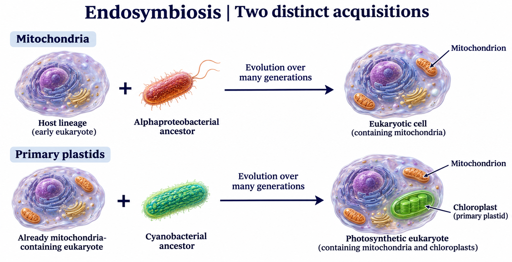
Two distinct acquisitions
Mitochondrial and primary-plastid origins are shown as separate evolutionary acquisitions.

Evidence from genes
Mitochondrial and plastid sequences connect these organelles with bacterial and cyanobacterial ancestry.


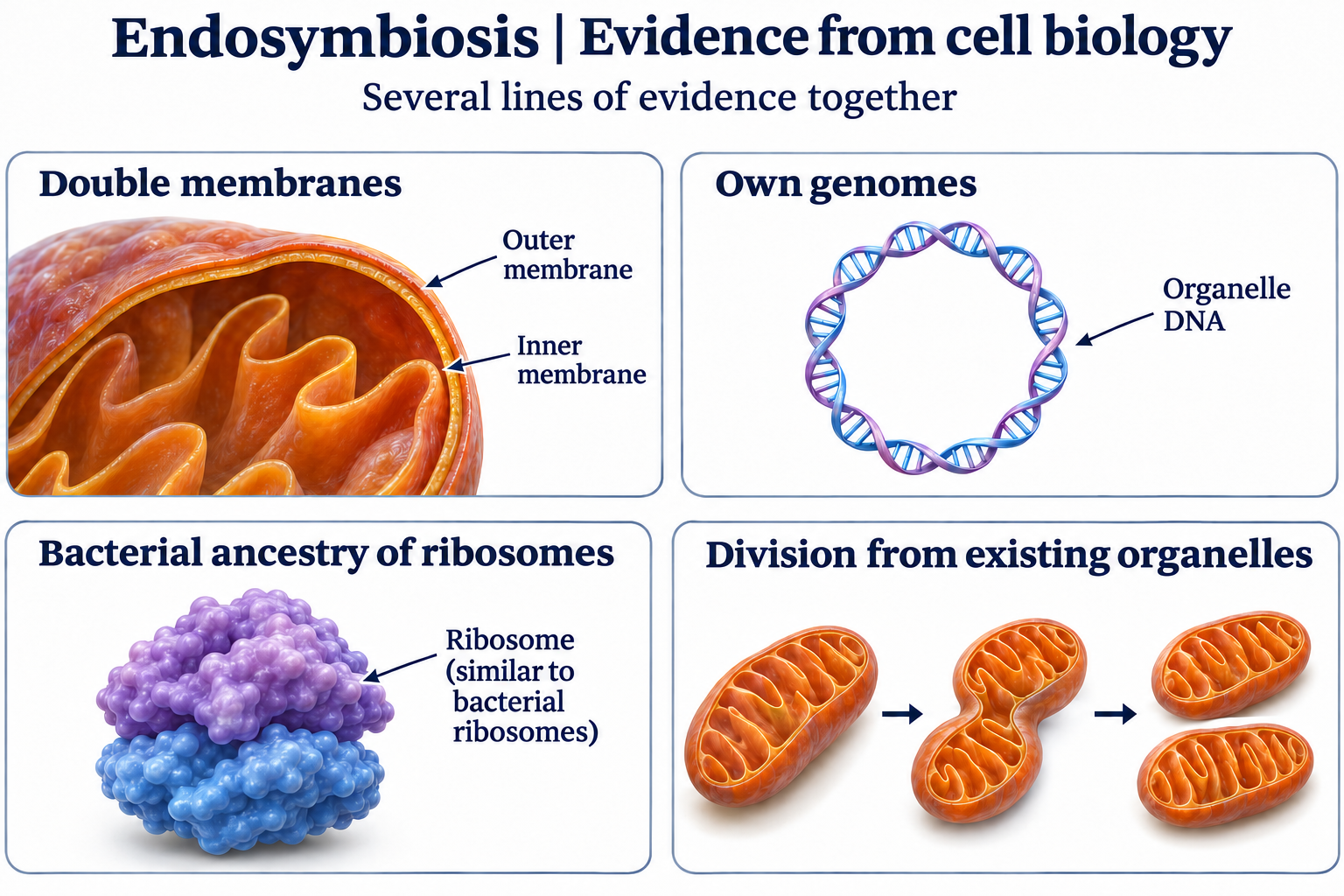
Evidence from cell biology
Membranes, genomes, ribosome ancestry and division provide complementary evidence for endosymbiosis.
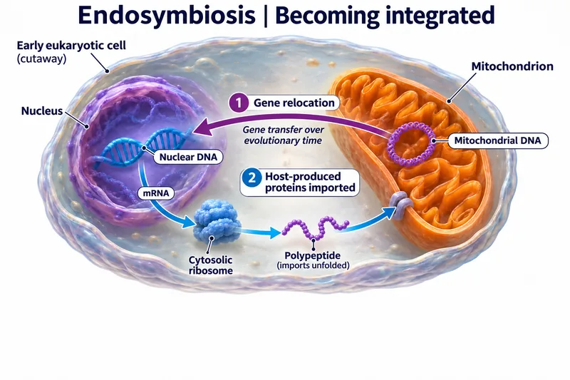
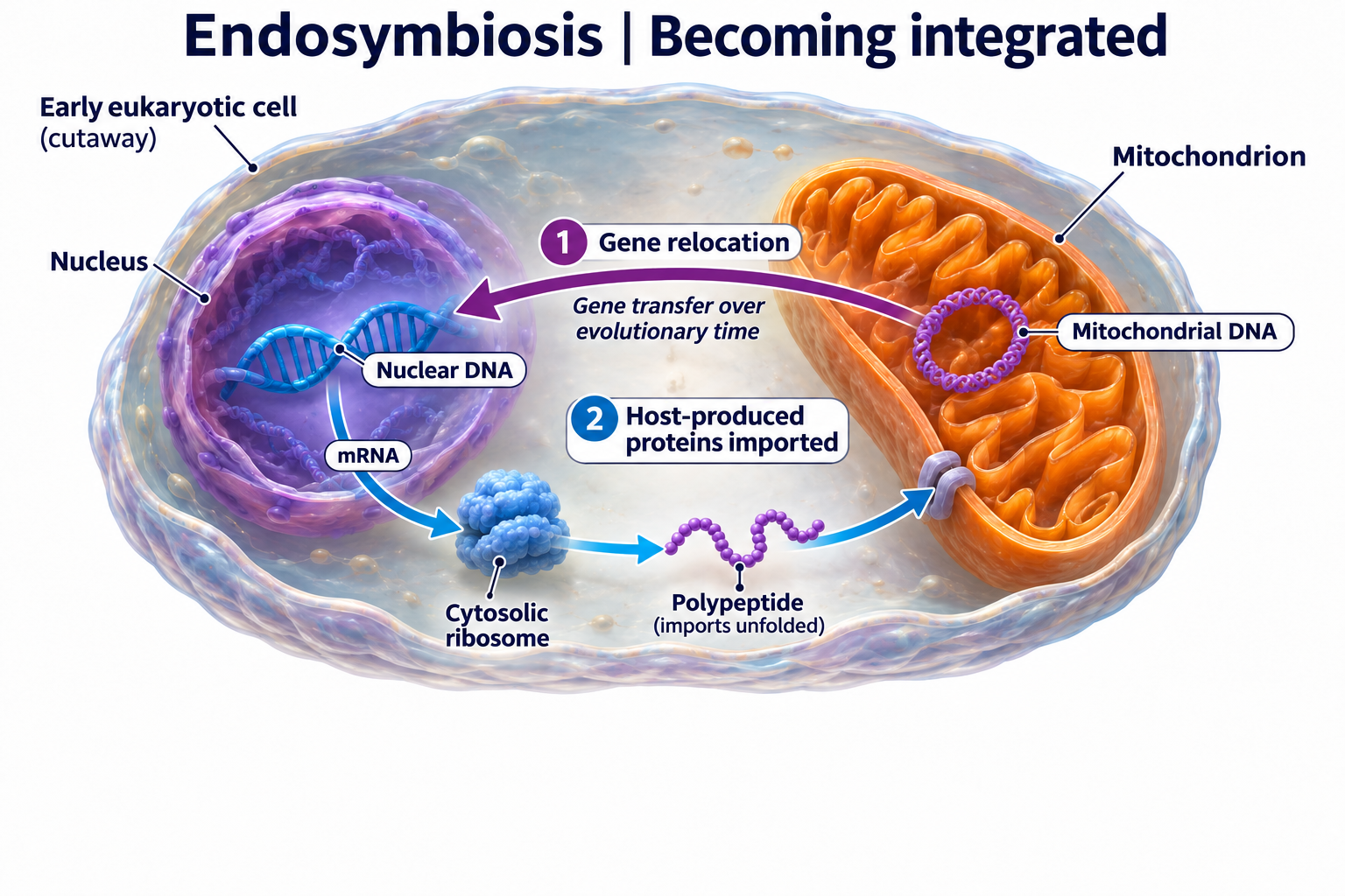
Becoming integrated
Gene relocation and import of host-produced proteins illustrate evolutionary integration of mitochondria.
 BIOLOGY · 5 VISUALSEnergy flow and matter cyclingDistinguish one-way energy transfer from the recycling of nutrients and carbon.
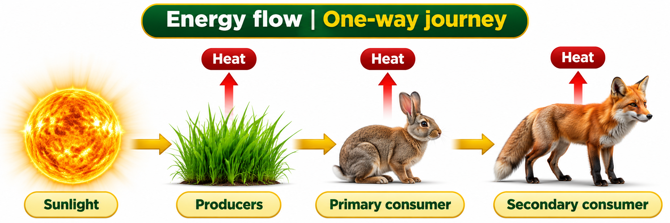
A one-way journey
Energy moves from sunlight through producers and consumers, with heat released along the way.

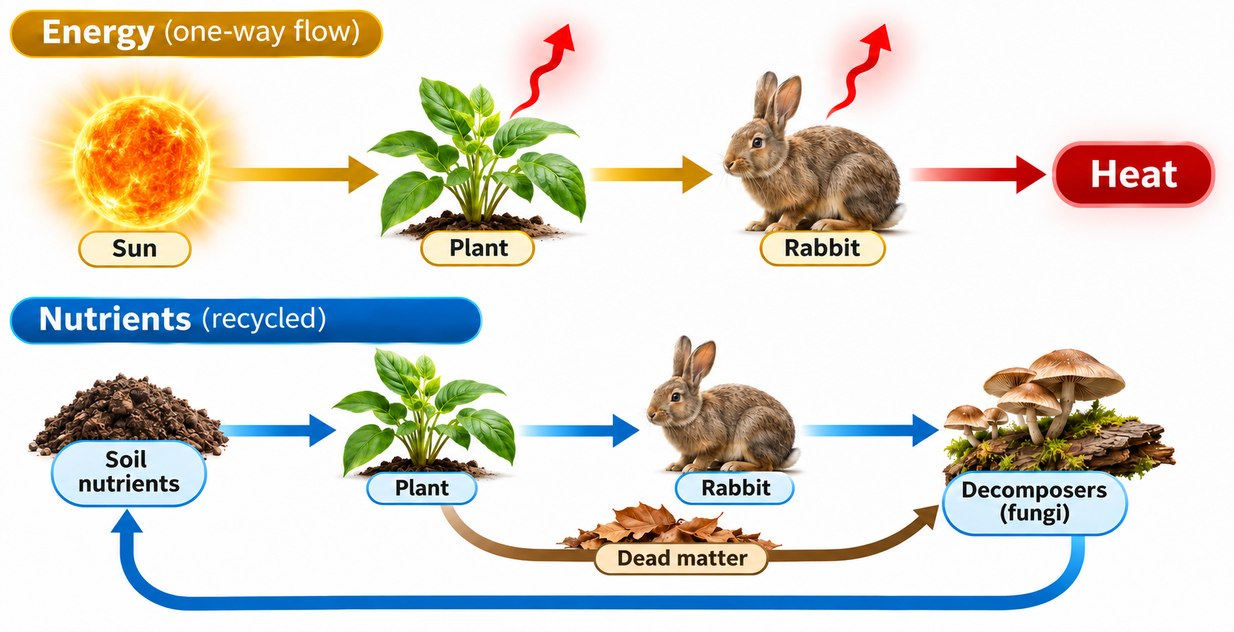
Energy versus nutrients
Energy flows through an ecosystem while nutrients return through decomposition and uptake.
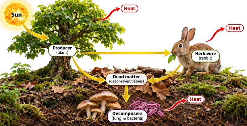
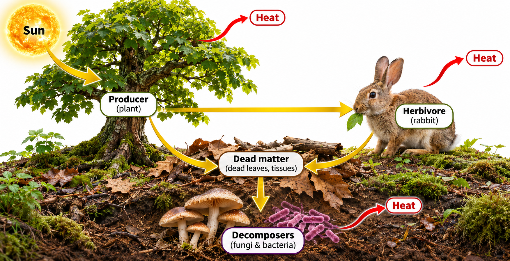
Decomposers and energy
A terrestrial example follows energy into herbivores and dead matter, with heat release from organisms.

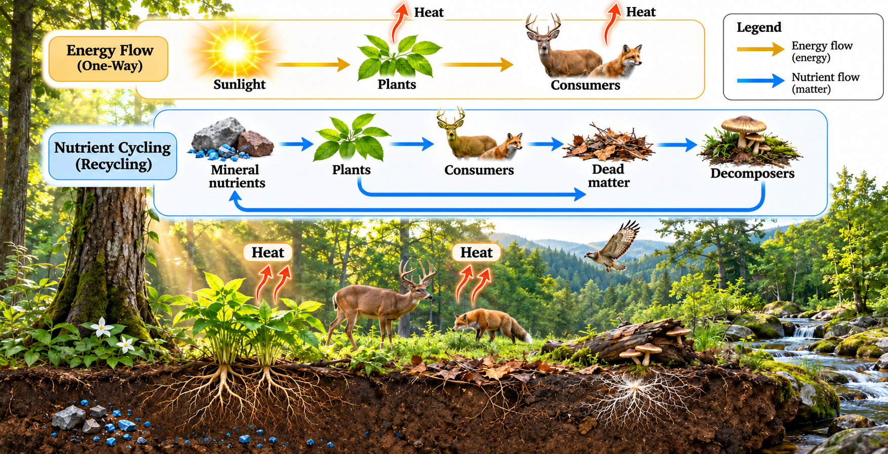
Flow and recycling together
A forest scene contrasts energy transfer with the cycling of mineral nutrients.

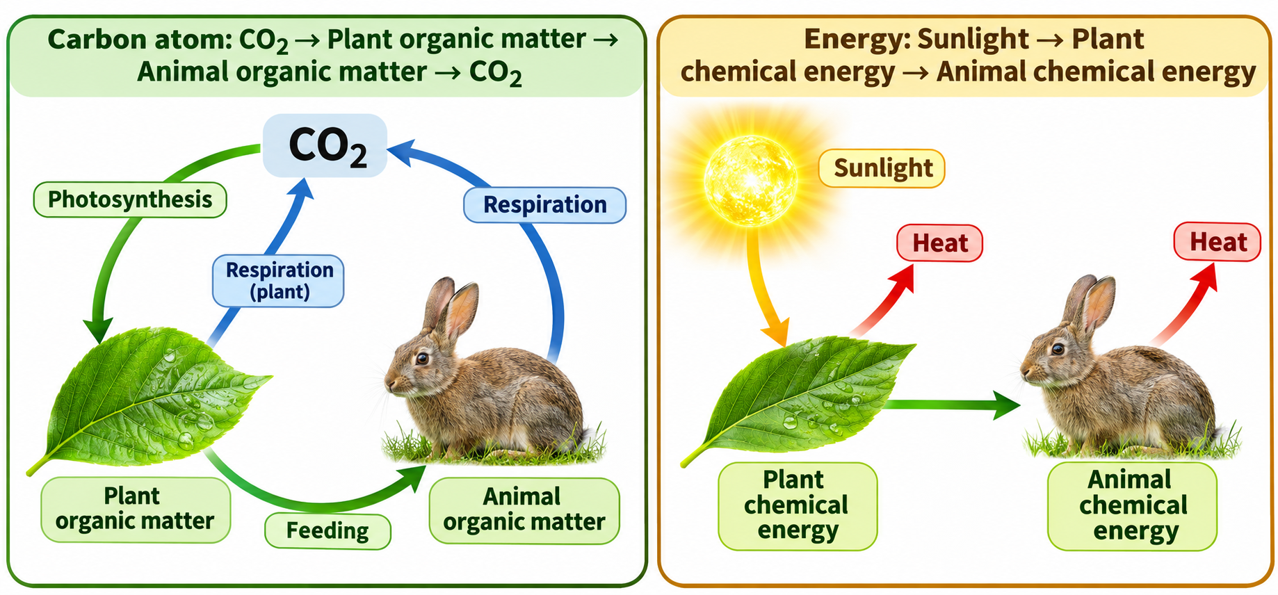
Follow carbon and energy
Side-by-side pathways distinguish a cycling carbon atom from sunlight-derived chemical energy.
 CHEMISTRY · 5 VISUALSVSEPR molecular shapesCompare electron-domain arrangements and molecular shapes, then connect shape with polarity.
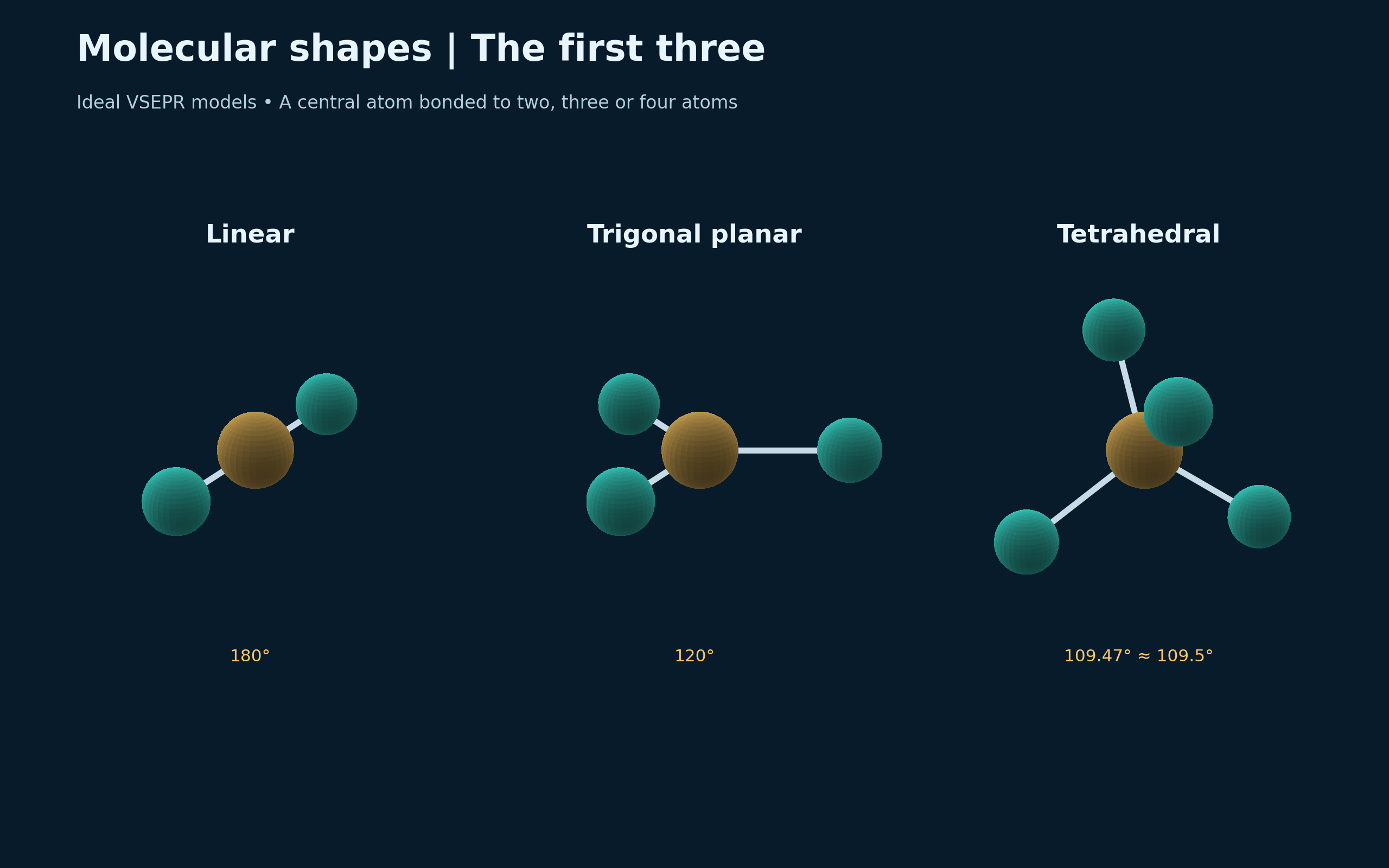
The first three shapes
Ideal models compare linear, trigonal planar and tetrahedral shapes with their bond angles.
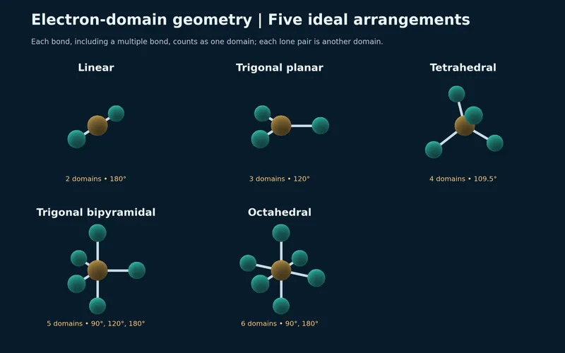
Five electron-domain arrangements
Models compare two through six electron domains: linear, trigonal planar, tetrahedral, trigonal bipyramidal and octahedral.


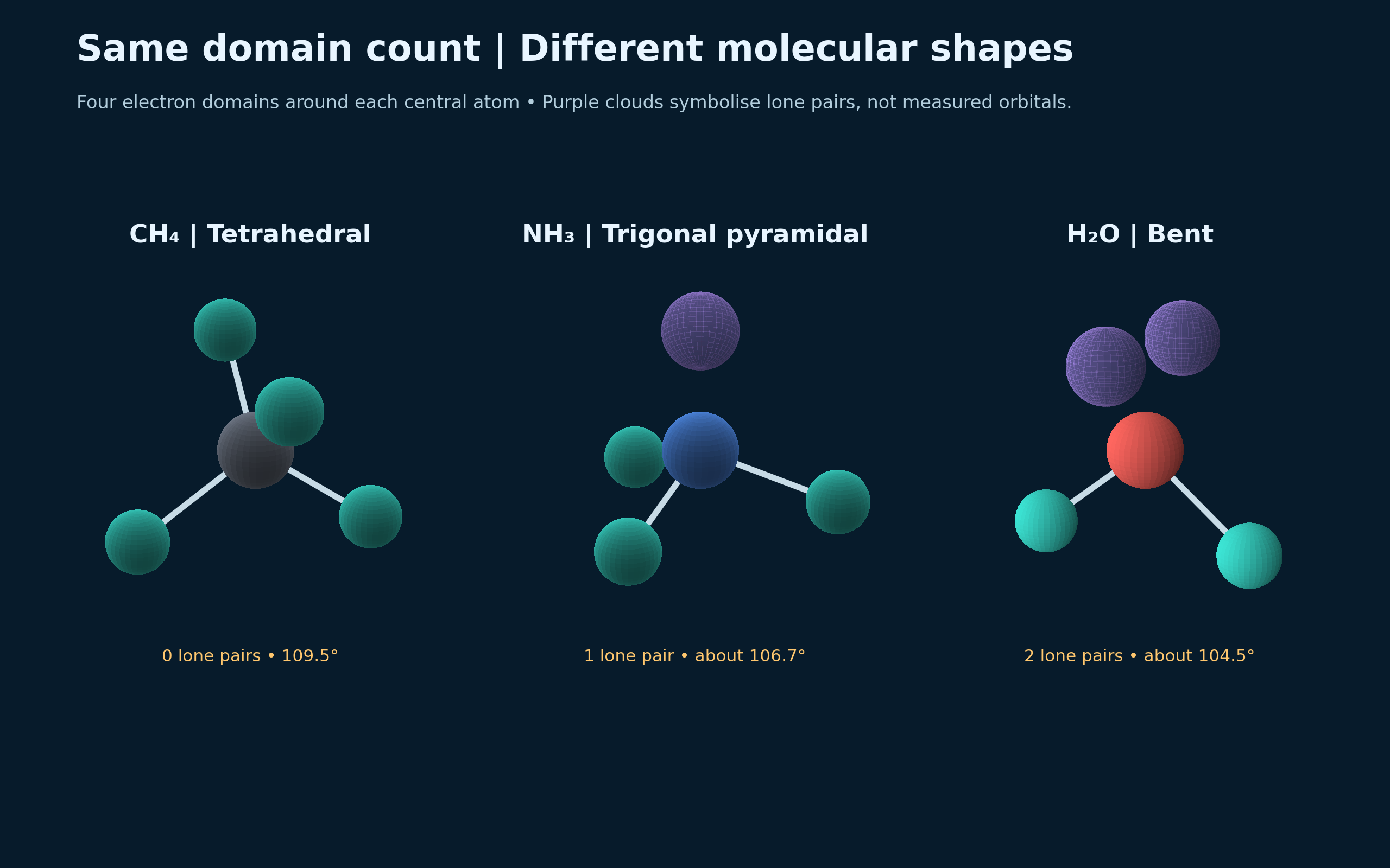
Same domain count, different shapes
Methane, ammonia and water illustrate the effect of lone pairs on molecular shape.

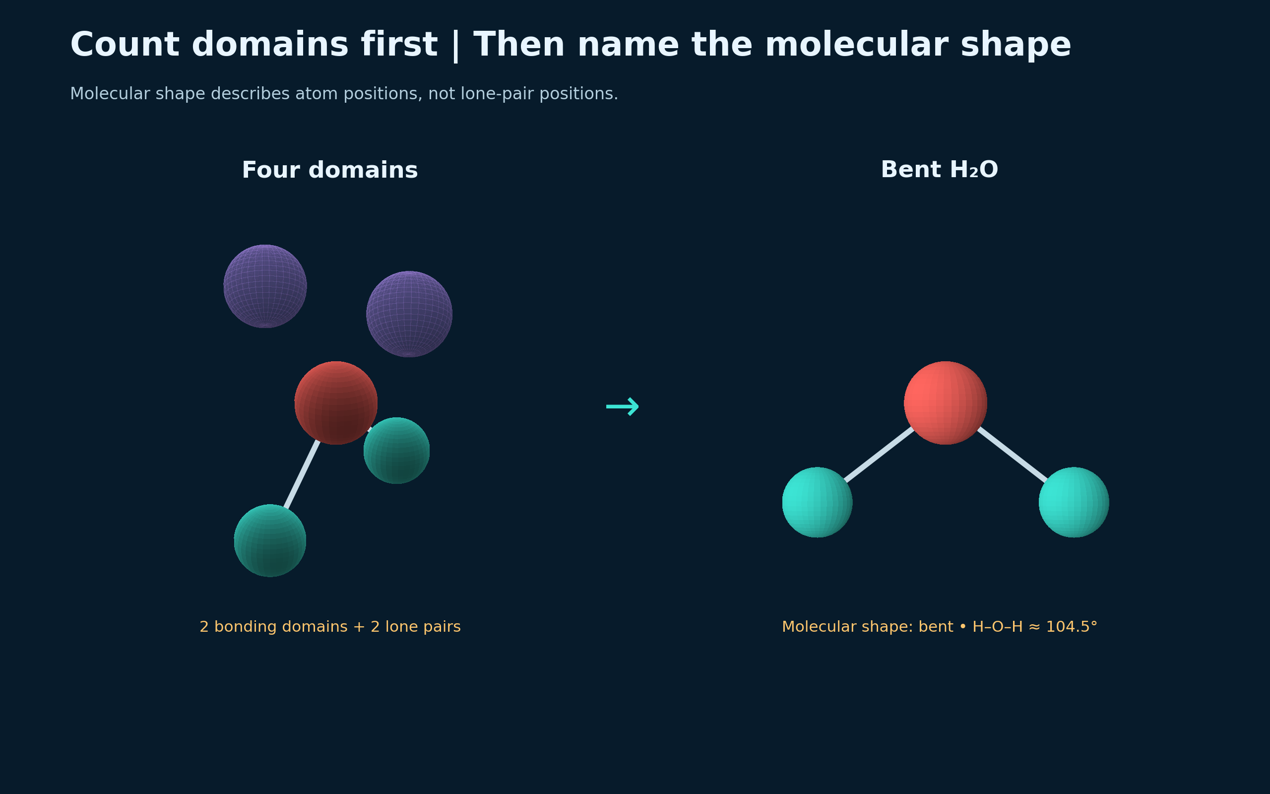
Count domains, then name the shape
A water model separates its four electron domains from the bent arrangement of its atoms.

Shape, symmetry and polarity
Carbon dioxide, methane and water connect molecular symmetry with dipole cancellation.

 CHEMISTRY · 5 VISUALSBond polarity versus molecular polarityDistinguish a polar bond from a polar molecule by combining bond dipoles in three dimensions.
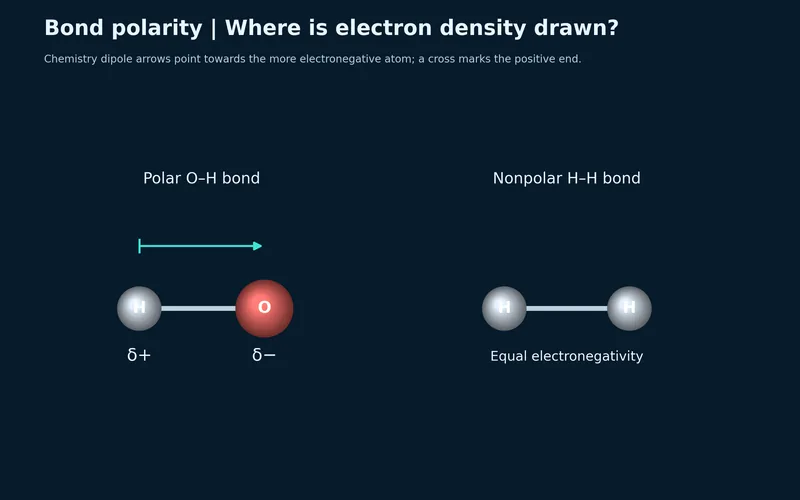
Where electron density is drawn
O–H and H–H bonds compare unequal and equal electron sharing.


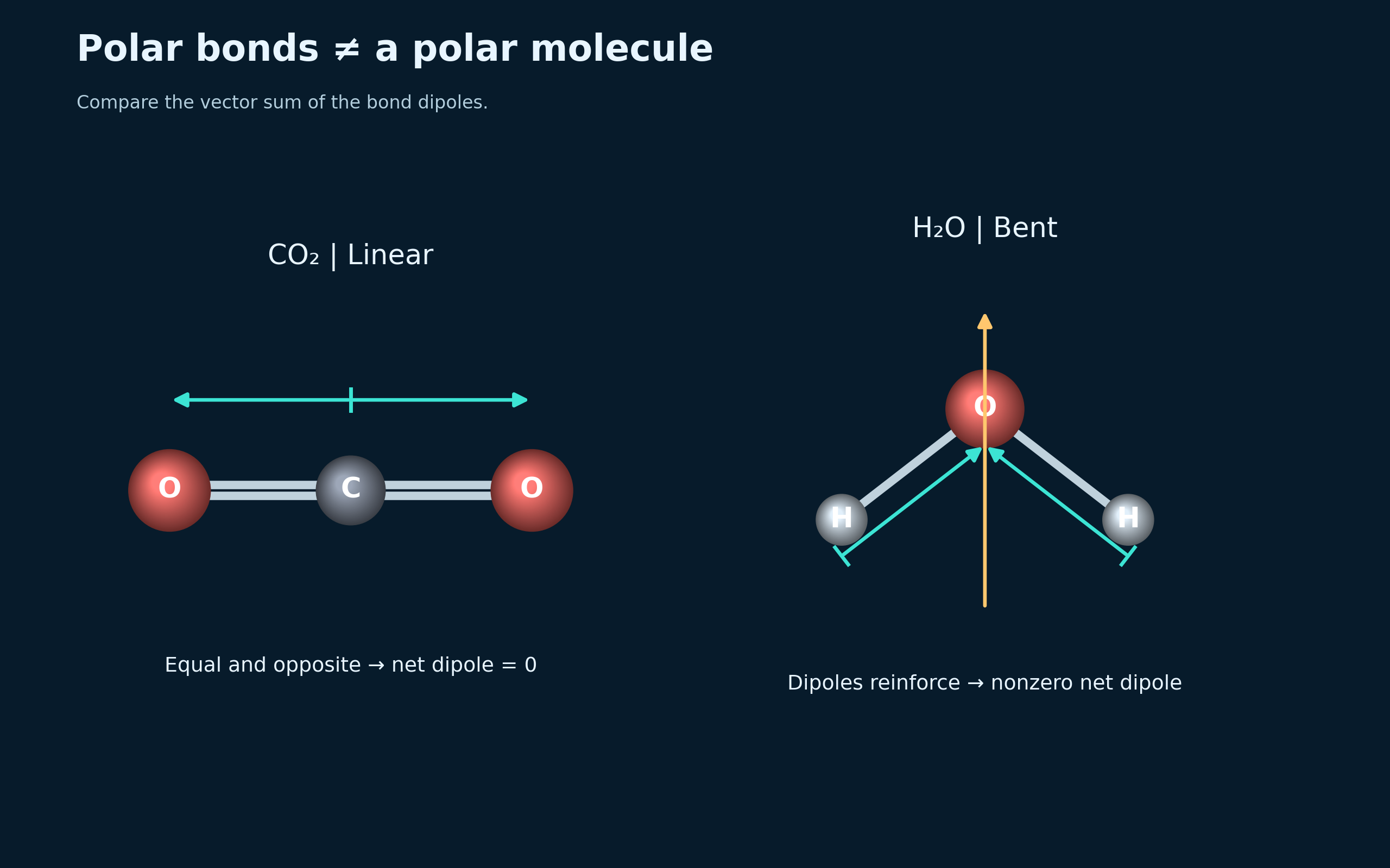
Polar bonds need not make a polar molecule
Opposing carbon dioxide dipoles cancel, while water has a nonzero resultant dipole.

Add the vectors
A water model and vector construction show cancelling sideways components and a resultant toward oxygen.

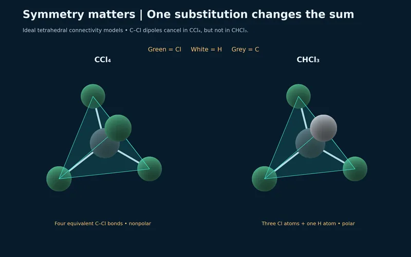
One substitution changes the sum
Tetrahedral carbon tetrachloride and chloroform compare symmetric and asymmetric bond arrangements.


Two questions about polarity
Carbon dioxide and water summarise the need to consider both bond polarity and molecular shape.

 CHEMISTRY · 5 VISUALSHydrogen bonding in waterExplore hydrogen bonding between water molecules and contrast it with the covalent bonds inside each molecule.
One hydrogen bond
Two water molecules show an intermolecular hydrogen bond beside intramolecular O–H bonds.


Donor and acceptor
Partial charges identify a donor O–H group and an oxygen acceptor in hydrogen bonding.


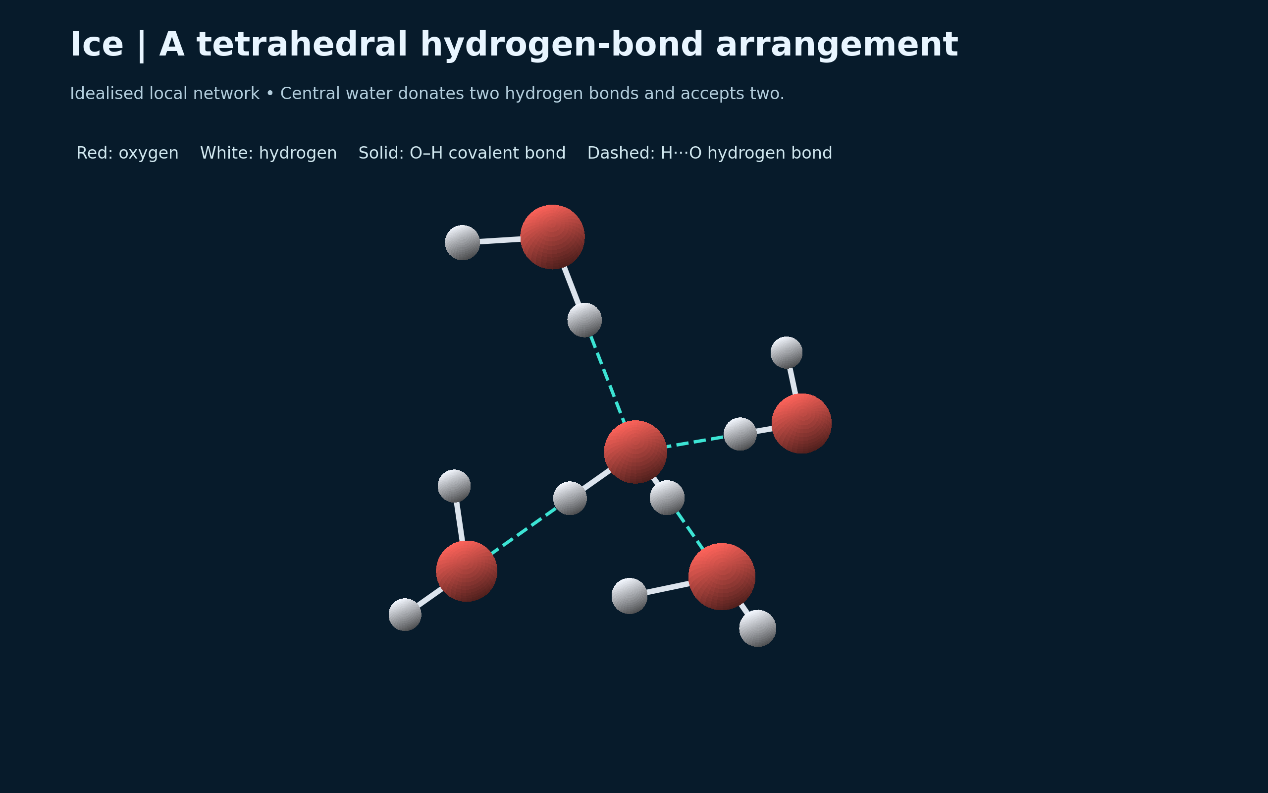
A tetrahedral arrangement in ice
An idealised local ice network shows a central water molecule donating two and accepting two hydrogen bonds.
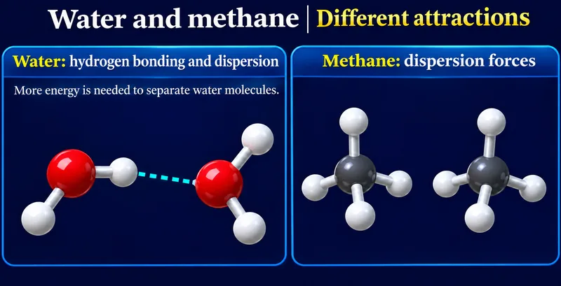
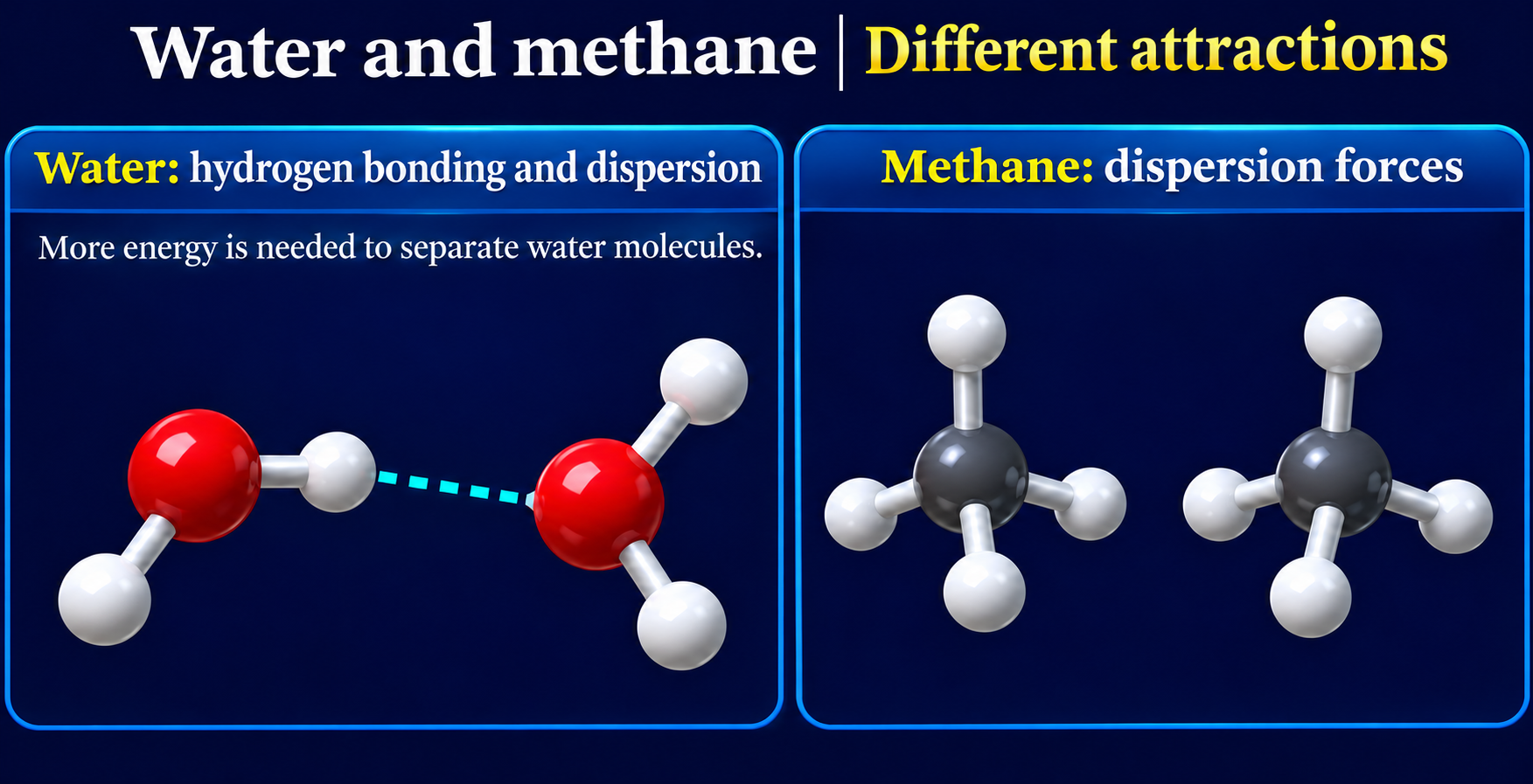
Water and methane
Molecular examples contrast hydrogen bonding and dispersion in water with dispersion in methane.

A changing network
A conceptual liquid-water snapshot shows a hydrogen-bond network that continually forms and breaks.

 CHEMISTRY · 5 VISUALSSodium chloride ionic latticeExplore the extended sodium chloride lattice, coordination and the movement of ions when molten.
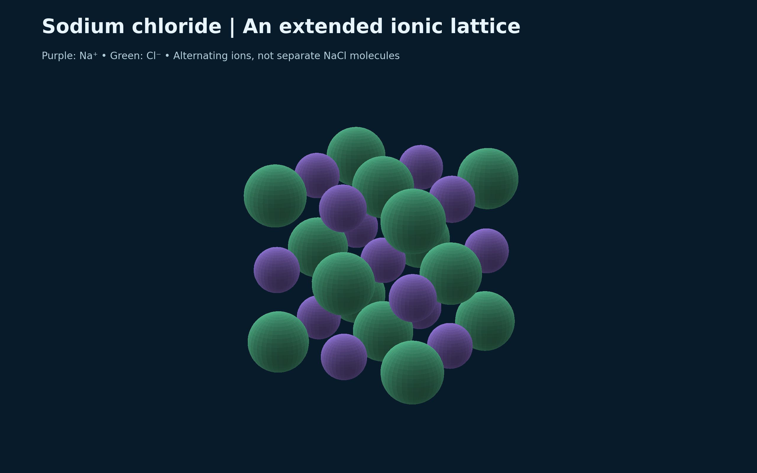
An extended ionic lattice
Alternating sodium and chloride ions form a repeating lattice rather than separate NaCl molecules.

Six nearest neighbours
A central sodium ion is surrounded octahedrally by six chloride ions.


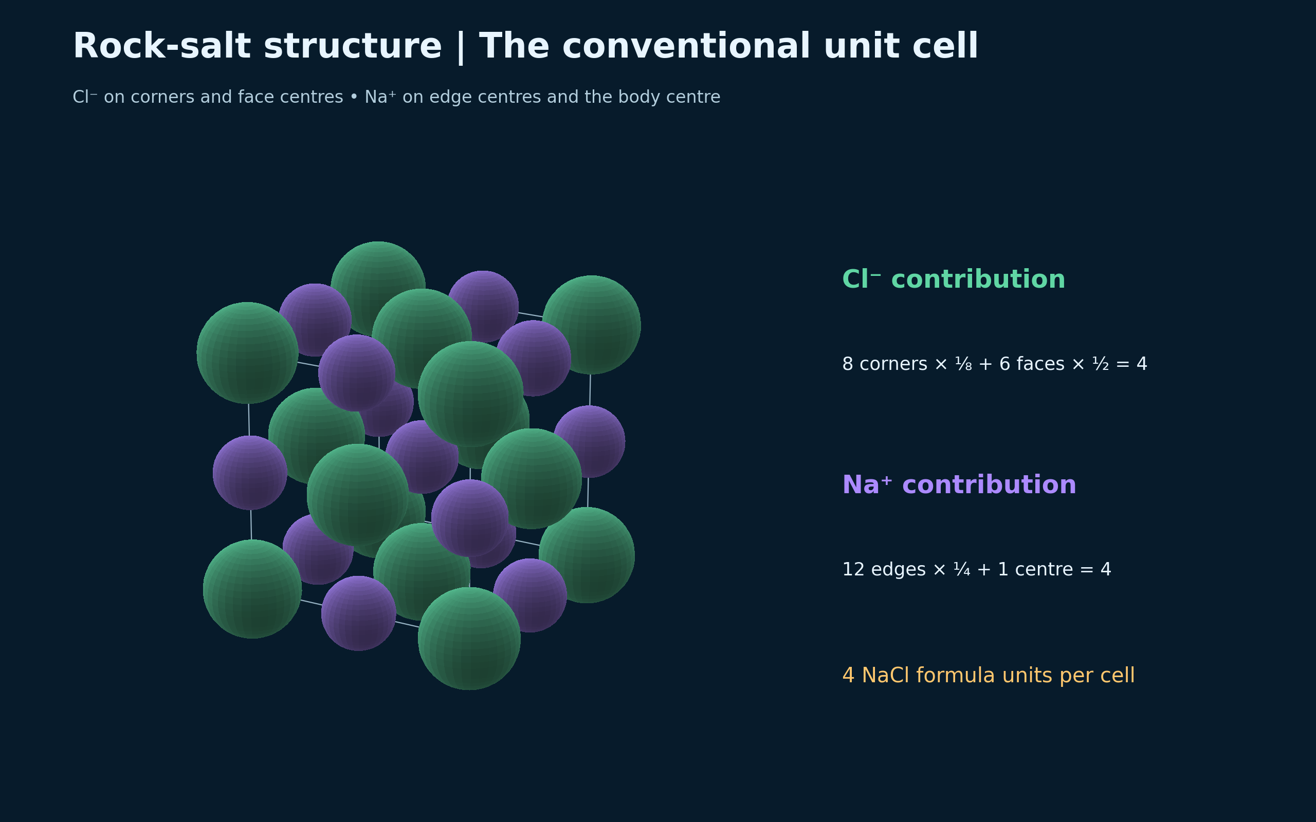
The conventional unit cell
Corner, face, edge and centre contributions give four NaCl formula units per conventional cell.

Solid and molten salt
Fixed lattice positions are compared with mobile ions drifting in molten sodium chloride.


Coordination in three dimensions
A larger ideal rock-salt lattice shows repeated sixfold coordination.

 CHEMISTRY · 5 VISUALSAtomic orbital shapesExplore orbital shapes, wavefunction phase and nodes using analytical hydrogenic models.
Spherical and directional orbitals
Hydrogenic 1s and 2p wavefunction surfaces compare spherical symmetry with two lobes and a nodal plane.

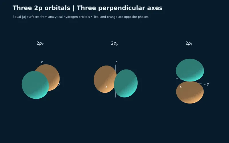
Three perpendicular 2p orbitals
Three equal-magnitude hydrogenic wavefunction surfaces show 2px, 2py and 2pz orientations.


A radial node changes phase
Equatorial slices compare 1s with the radial node in 2s, using colour for phase and brightness for wavefunction magnitude.

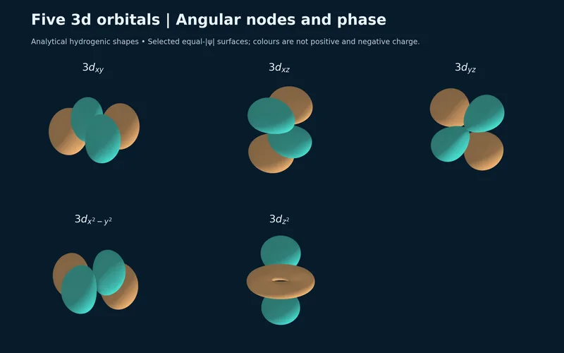
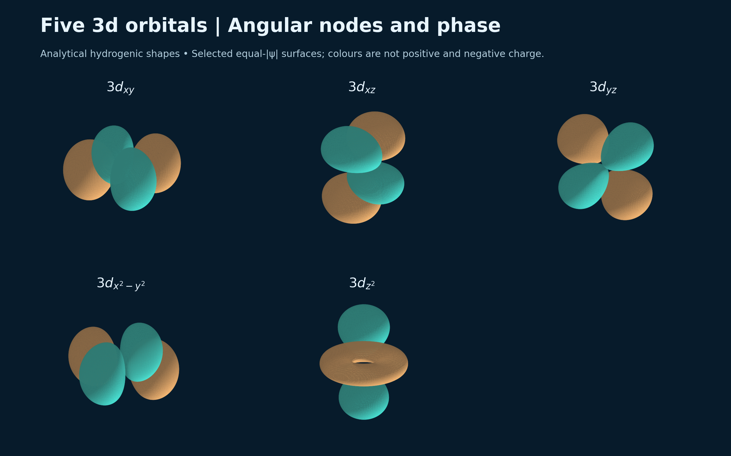
Five 3d orbitals
Analytical hydrogenic surfaces compare the shapes and phases of five 3d orbitals.

Sigma and pi combinations
Conceptual p-orbital superpositions contrast end-on and side-on bonding overlap.

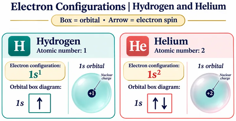 CHEMISTRY · 5 VISUALSElectron configurations and orbital fillingBuild electron configurations with orbital boxes, then consider exceptions and ion formation.
Hydrogen and helium
Orbital boxes compare one electron in hydrogen with paired opposite spins in helium.

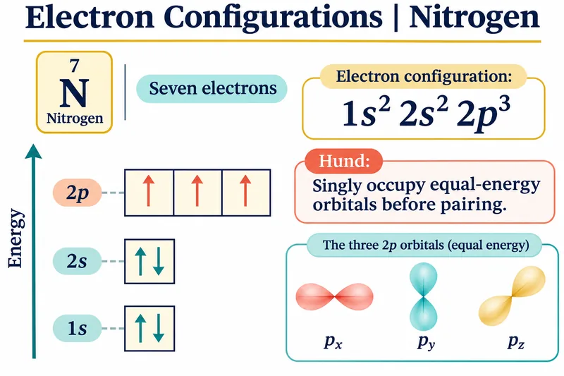
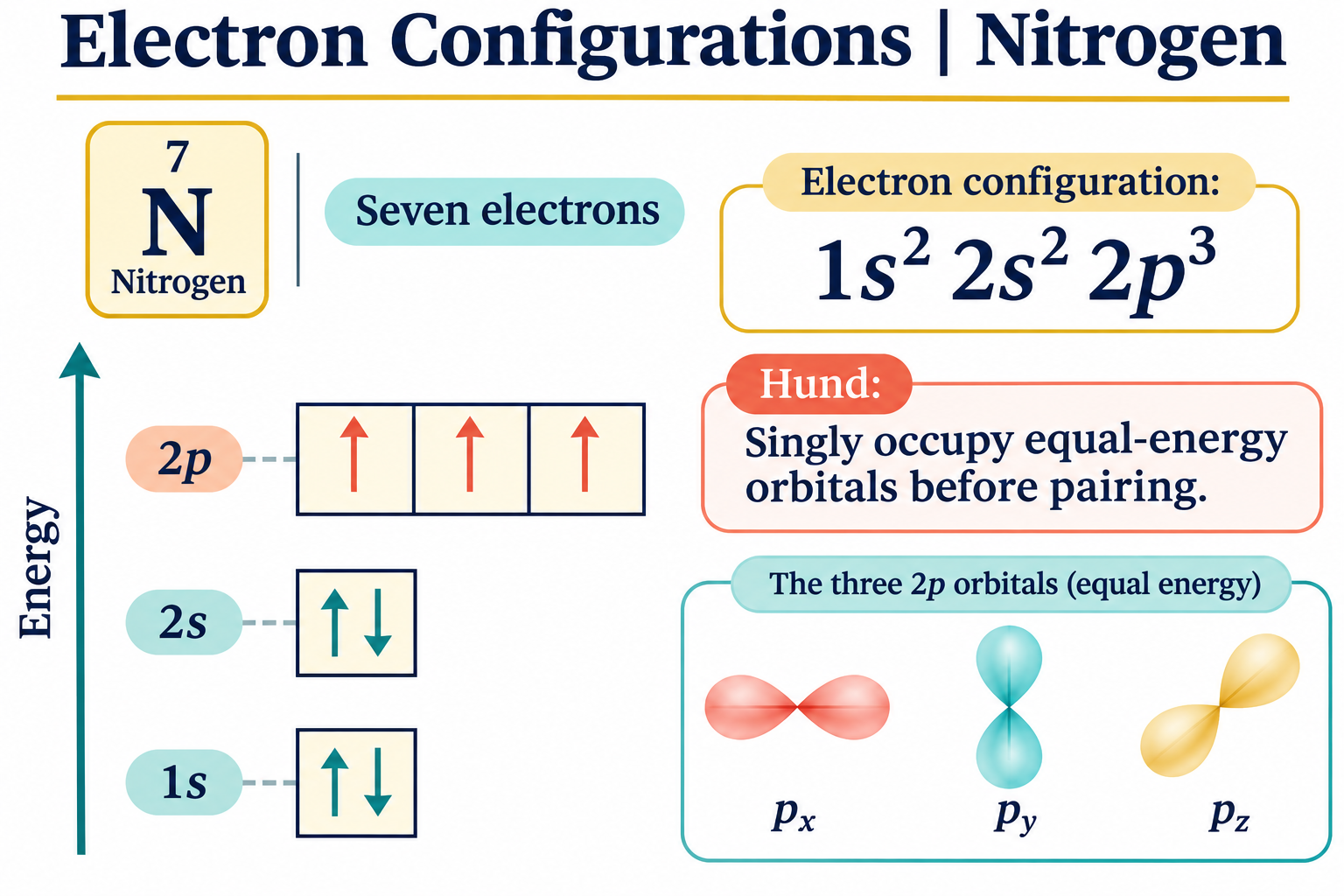
Nitrogen and Hund’s rule
Nitrogen’s seven electrons occupy 1s, 2s and three singly filled 2p orbitals.

Three filling principles
Aufbau, Pauli and Hund rules summarise a useful ground-state building method with exceptions.

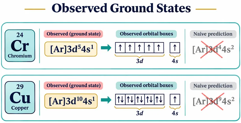
Chromium and copper exceptions
Observed chromium and copper configurations are compared with naive filling predictions.

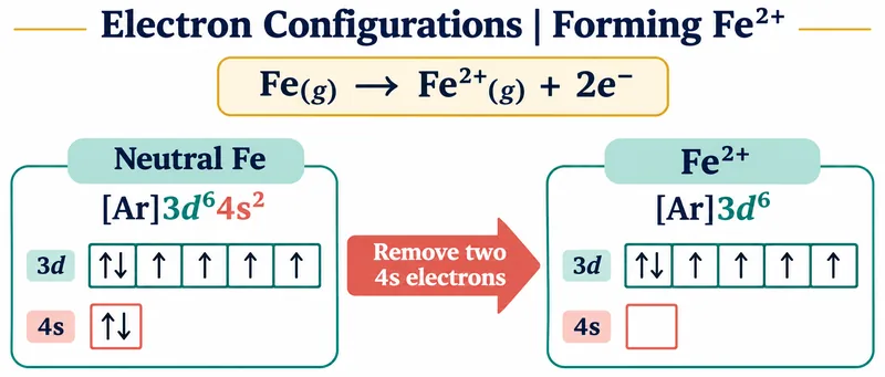
Forming Fe2+
An iron orbital diagram removes two 4s electrons to leave the [Ar]3d6 configuration.

 CHEMISTRY · 5 VISUALSAtomic radius trendsConnect qualitative atomic-radius trends with occupied shells, nuclear attraction and definitions of radius.
A periodic pattern
Qualitative sphere sizes show larger atoms down a group and generally smaller atoms across a period.

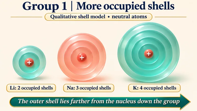
More occupied shells
Lithium, sodium and potassium shell models illustrate increasing occupied shells down Group 1.

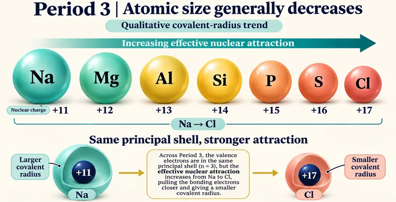
Period 3 size trend
Sodium through chlorine illustrate a qualitative covalent-radius decrease across the period.

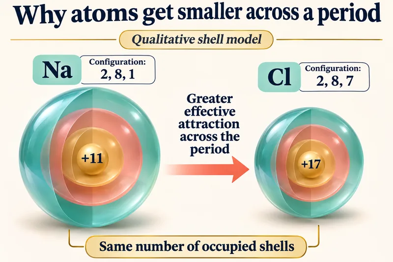
The same shell, stronger attraction
Sodium and chlorine shell models compare electron configurations and effective nuclear attraction.

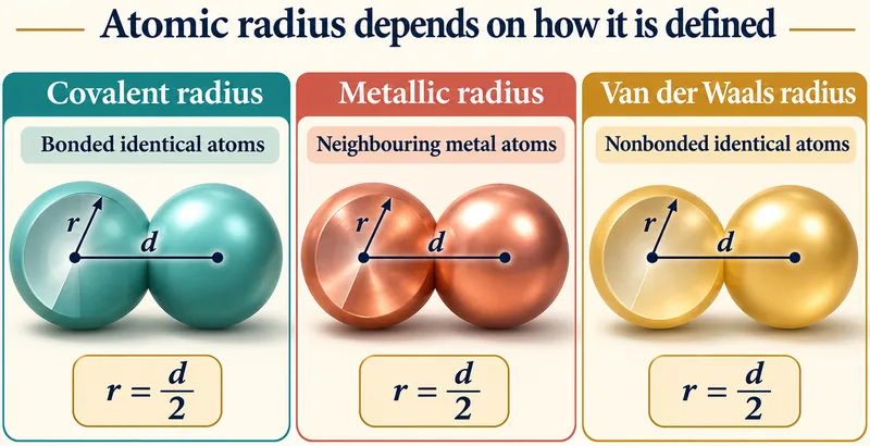
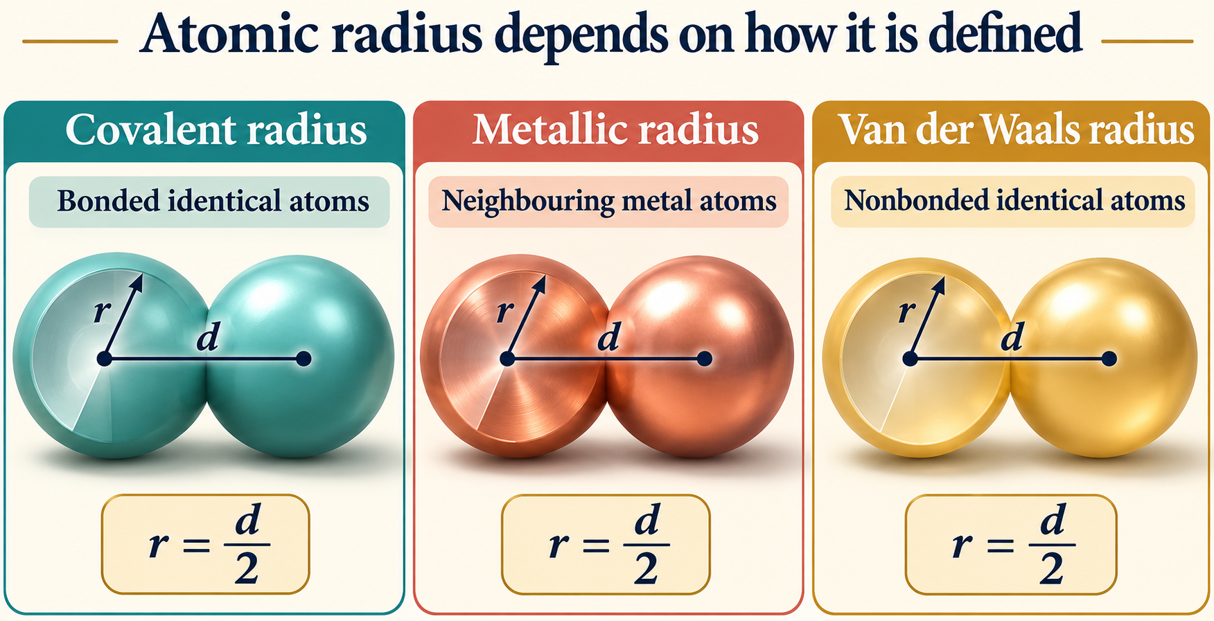
Radius depends on its definition
Covalent, metallic and van der Waals radii are each related to half a relevant internuclear distance.
 CHEMISTRY · 5 VISUALSFirst ionization energy trendsExplain first-ionisation-energy patterns and their exceptions using electron configurations.
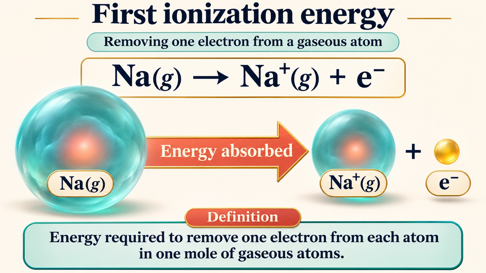
Removing a gaseous electron
A sodium example defines first ionisation energy and shows energy absorption.
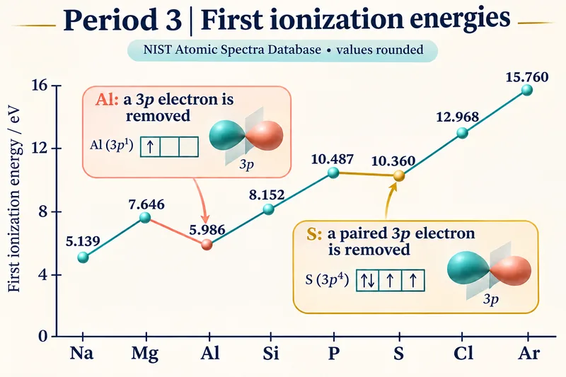
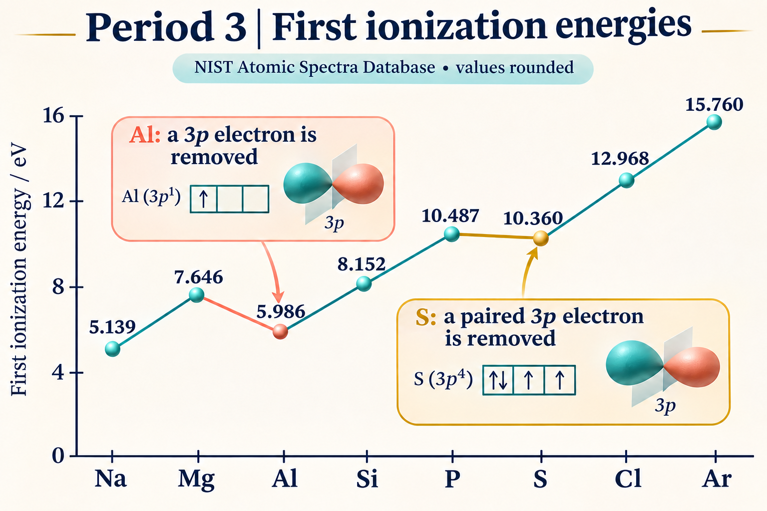
Period 3 energies
A graph of rounded NIST values shows the Period 3 trend and the aluminium and sulfur dips.

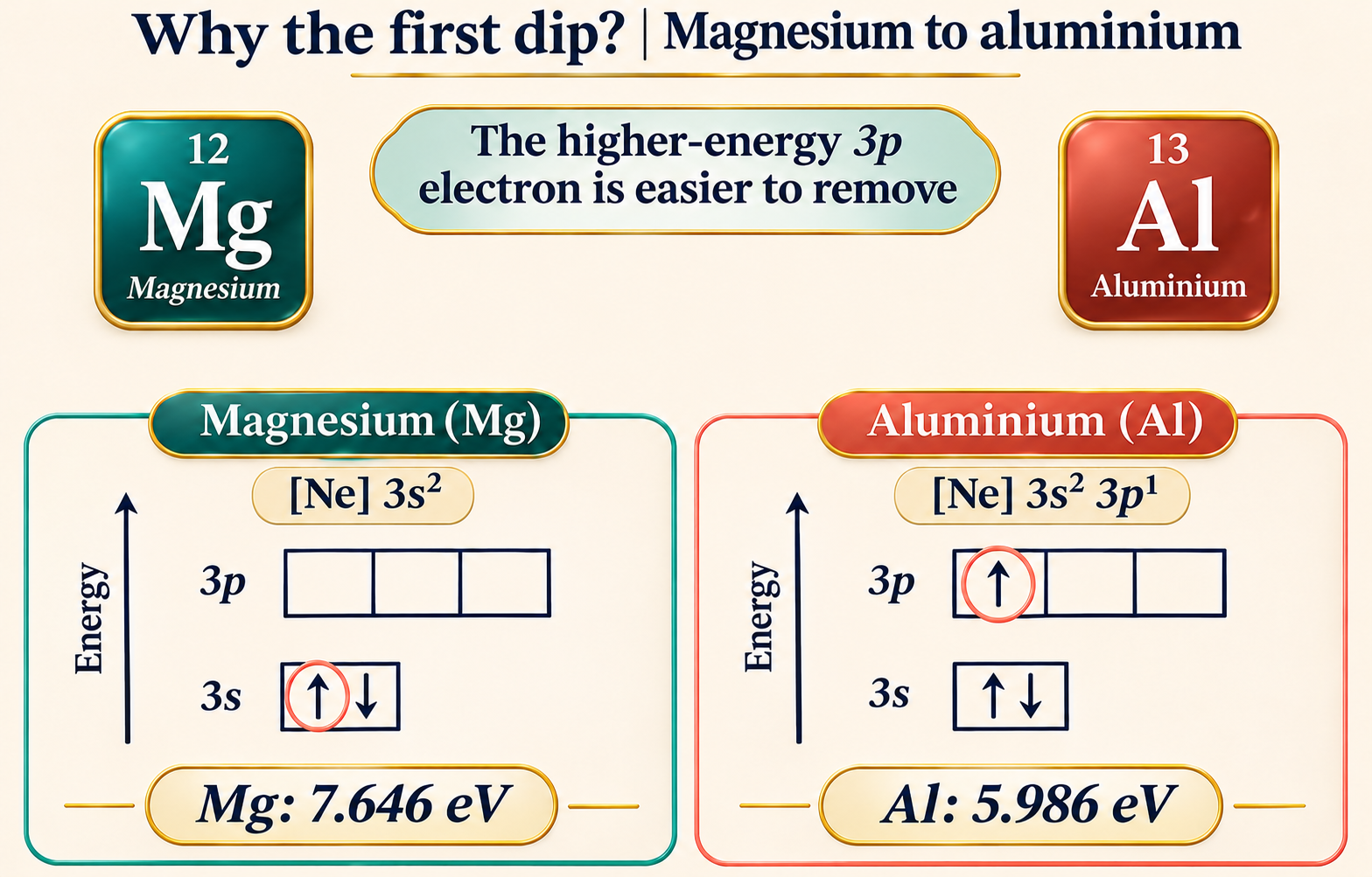
Magnesium to aluminium
Orbital boxes show that aluminium loses a higher-energy 3p electron rather than a 3s electron.

Phosphorus to sulfur
Paired-electron repulsion helps explain sulfur’s slightly lower first ionisation energy.


A jump after two electrons
Successive magnesium ionisation energies show the large increase on removing an inner-shell electron.

 CHEMISTRY · 5 VISUALSLimiting reactant and excess reactantIdentify the limiting reactant by counting complete reaction sets and relating them to mole ratios.
The reactant that runs out
Four hydrogen molecules and one oxygen molecule produce two waters with hydrogen left over.


Count complete reaction sets
Six hydrogen and two oxygen molecules make two complete reaction sets and leave two hydrogen molecules.


Conservation of atoms
Product and excess-reactant particles preserve all twelve hydrogen and four oxygen atoms.


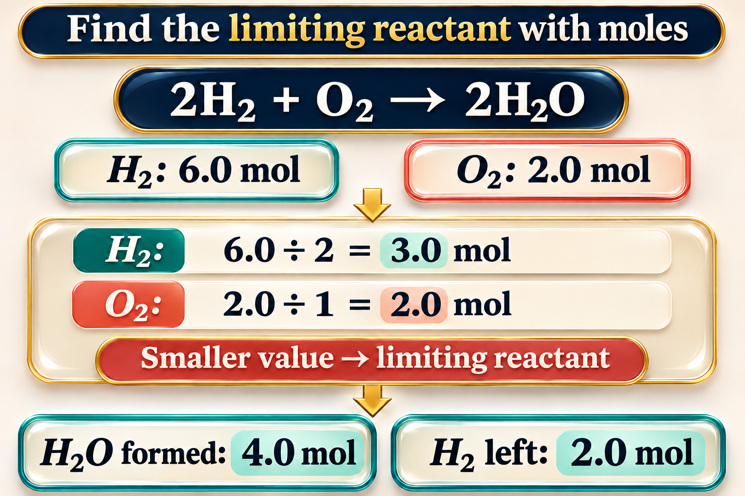
Use mole ratios
A worked calculation compares amount divided by coefficient to identify oxygen as limiting.

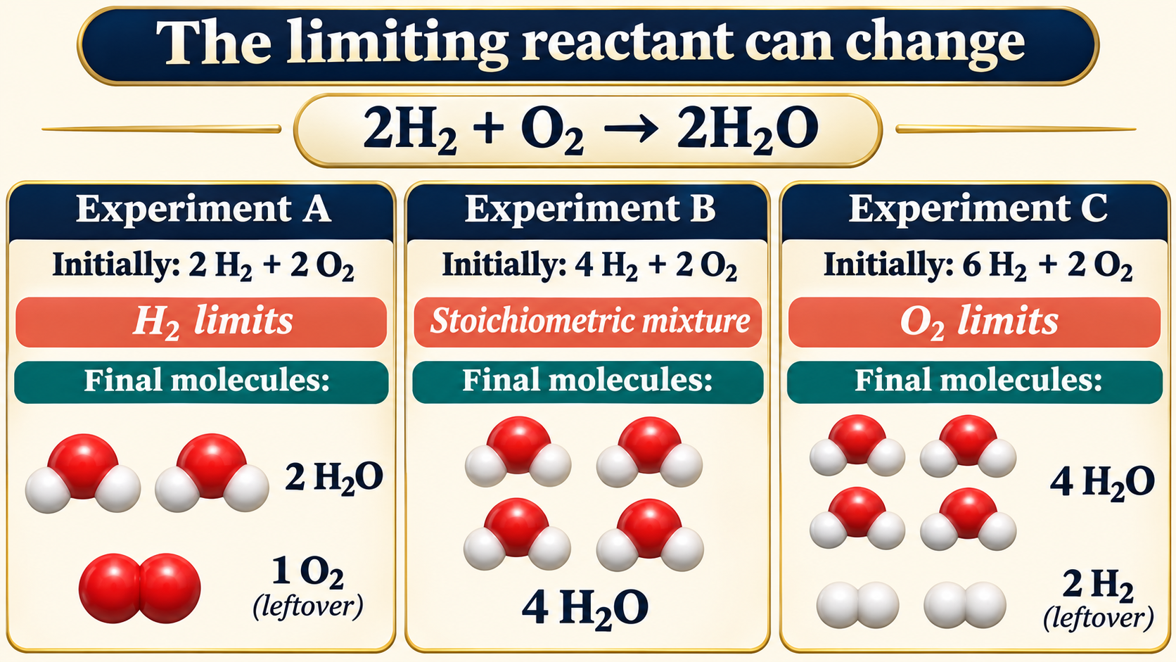
The limiting reactant can change
Three starting mixtures compare hydrogen-limited, stoichiometric and oxygen-limited cases.
 CHEMISTRY · 5 VISUALSBalancing equations with particle modelsBalance chemical equations by conserving atoms and charge, without changing chemical formulae.
Keep every atom
A water-formation equation and particle count show conservation of hydrogen and oxygen atoms.

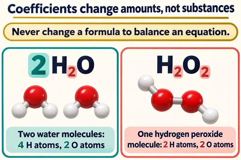
Amounts, not substances
Two water molecules are contrasted with one hydrogen peroxide molecule to distinguish coefficients from subscripts.


Methane combustion
Particle models and a count table verify the balanced methane combustion equation.

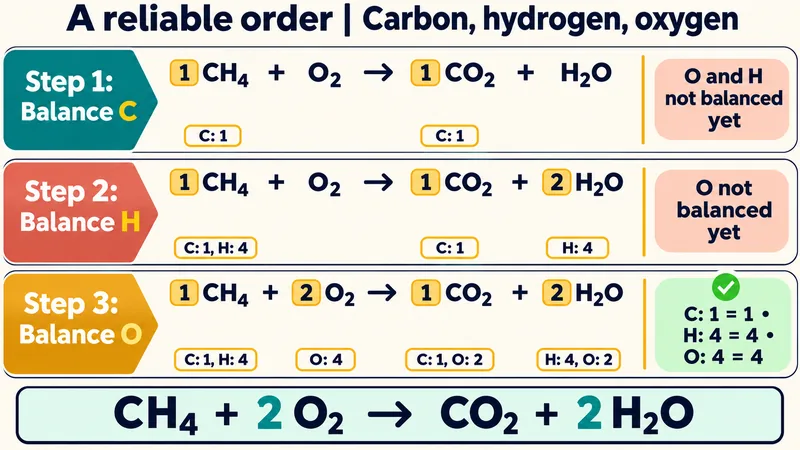
Carbon, hydrogen, then oxygen
A staged example balances methane combustion one element at a time.


Charge must balance too
Iron oxidation and chlorine reduction half-equations combine with conserved total charge.

 CHEMISTRY · 5 VISUALSThe mole: equal numbers, different massesConnect amount in moles with specified entities, molar mass and sample mass.
Counting specified entities
One mole of carbon atoms, copper atoms and water molecules represents the same specified-entity count.
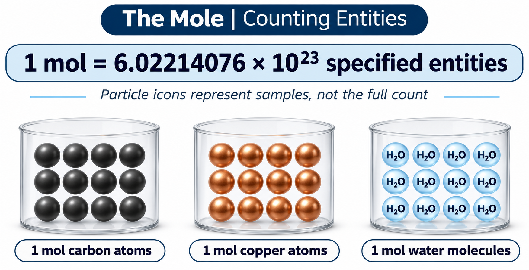

Equal counts, different masses
Graphite, copper and water samples compare approximate masses for one mole of their specified entities.
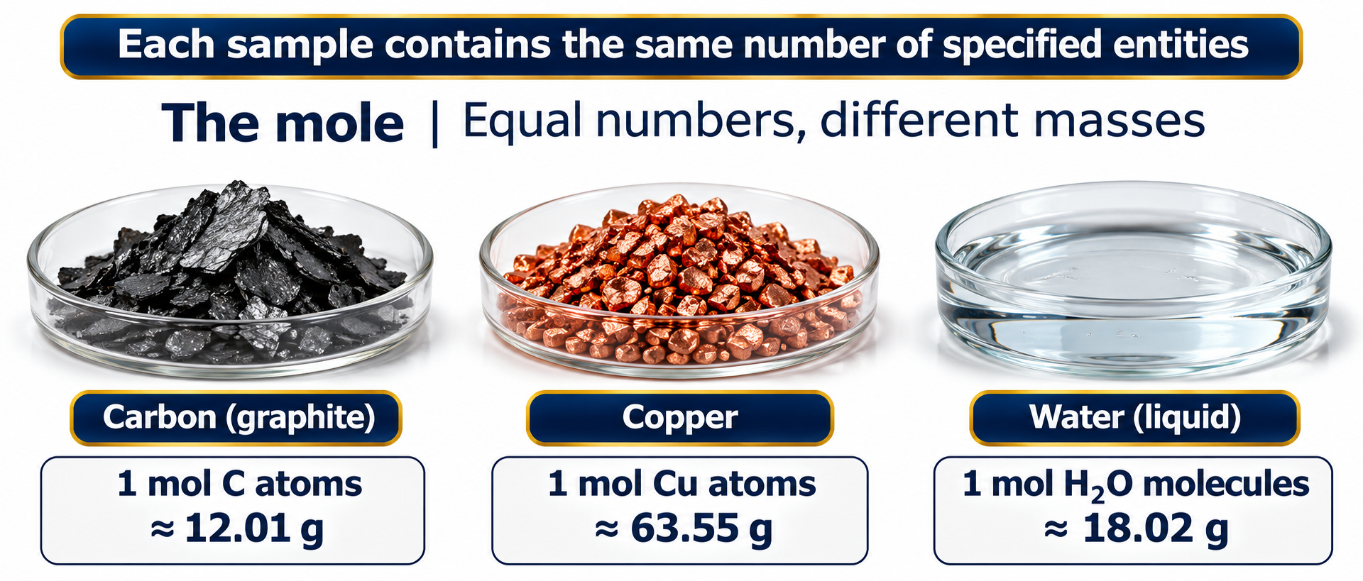

Two useful relationships
A relationship map connects number of entities, amount in moles and mass.

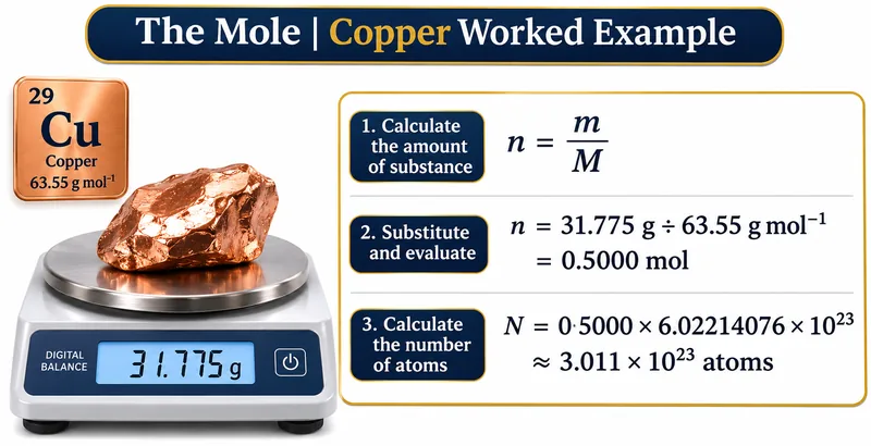
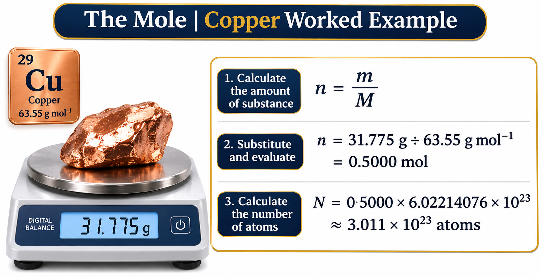
A copper calculation
A worked example converts 31.775 g of copper to 0.5000 mol and an atom count.

Scaling a sample
Copper amounts of 0.25, 0.50 and 1.00 mol show mass and atom number scaling together.

 CHEMISTRY · 5 VISUALSGalvanic cellFollow electron and ion movement through a zinc–copper galvanic cell.
The cell circuit
A zinc–copper cell shows the external electron path and a salt bridge between half-cells.


Oxidation and reduction
Zinc oxidation at the negative anode is paired with copper-ion reduction at the positive cathode.


Completing the circuit
A potassium nitrate salt bridge supplies anions toward the anode and cations toward the cathode.

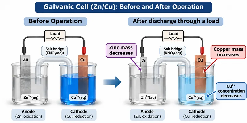
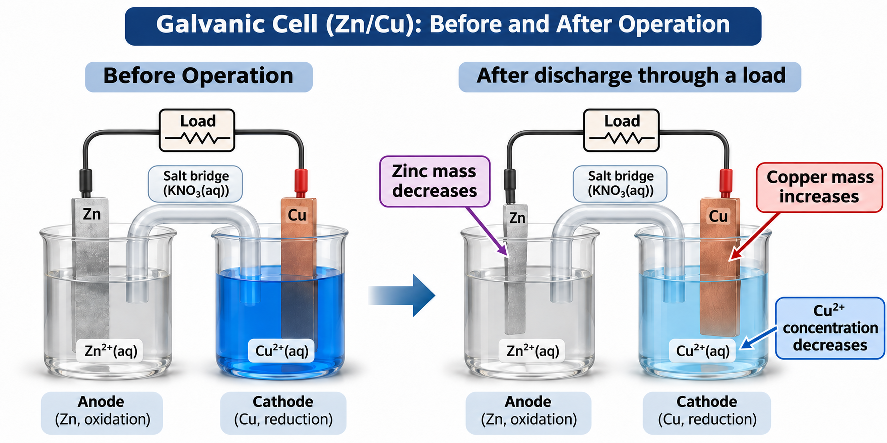
Before and after discharge
The zinc electrode loses mass while copper is deposited and copper-ion concentration falls.

The overall reaction
A zinc–copper cell combines half-reactions, cell notation and an approximate standard potential of 1.10 V.

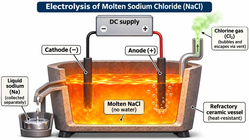 CHEMISTRY · 5 VISUALSElectrolysis of molten sodium chlorideExplain electrode reactions and charge transfer in molten sodium chloride, then compare with concentrated brine.
Molten sodium chloride
A conceptual cell identifies the negative cathode, positive anode and separated sodium and chlorine products.


Ions move to electrodes
Sodium ions move toward the cathode and chloride ions toward the anode in the molten electrolyte.

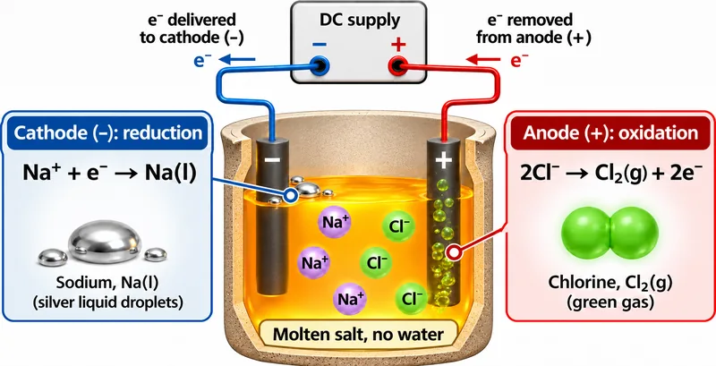
Half-equations and electrons
Electron delivery and removal are linked to sodium reduction and chloride oxidation.

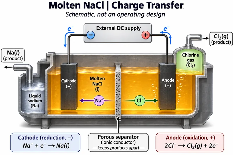
Charge transfer
A schematic cell separates electron flow through wires from ion movement through molten salt.

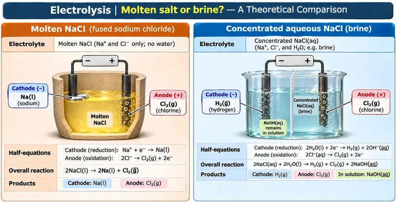
Molten salt or brine?
A theoretical comparison shows different cathode reactions in molten NaCl and concentrated aqueous NaCl.

 CHEMISTRY · 5 VISUALSStrong-acid and weak-acid titration curvesRead strong- and weak-acid titration curves and connect their shapes with buffer regions and equivalence points.
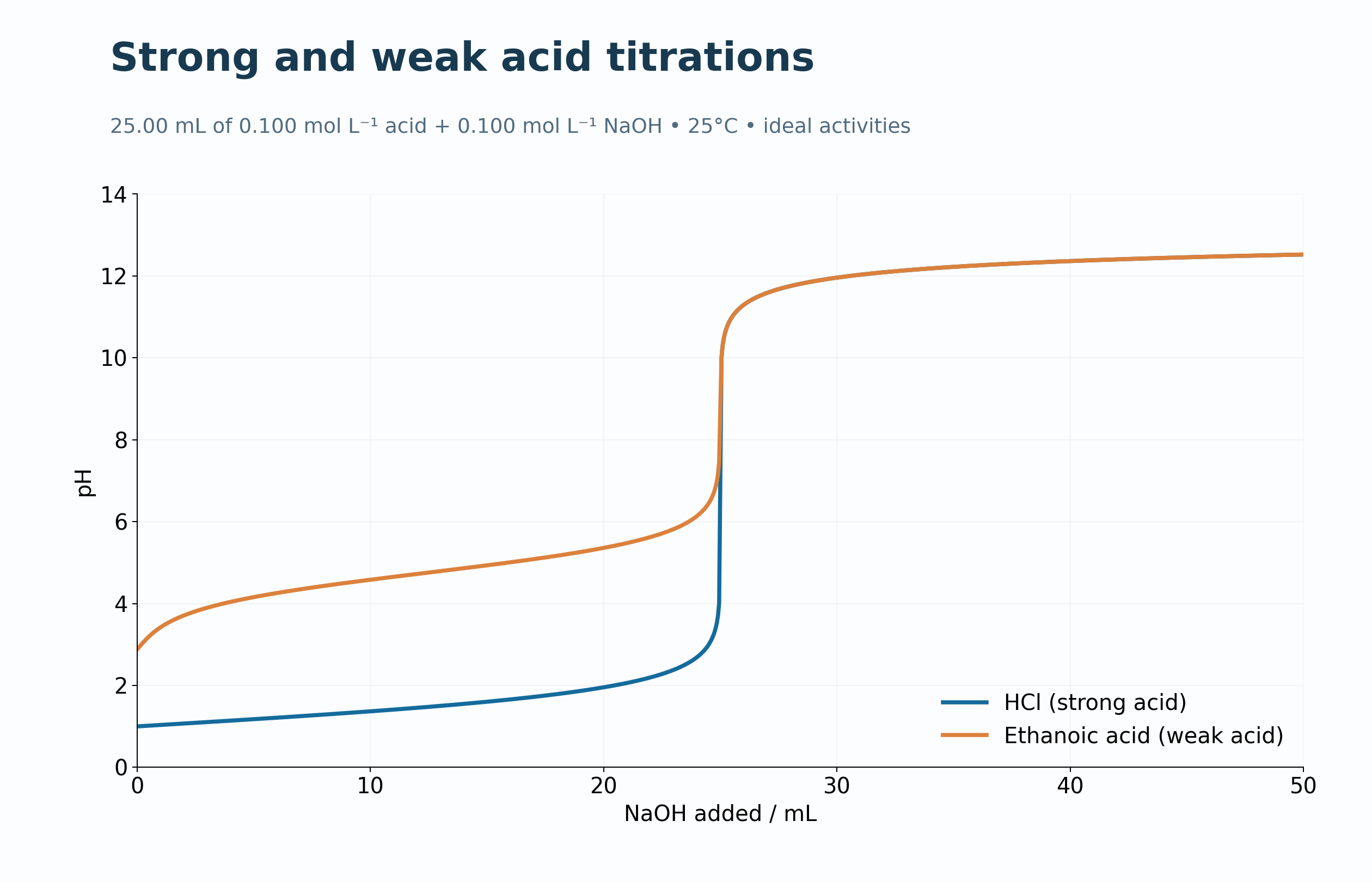
Strong and weak acids
Model curves compare hydrochloric and ethanoic acids titrated with sodium hydroxide.

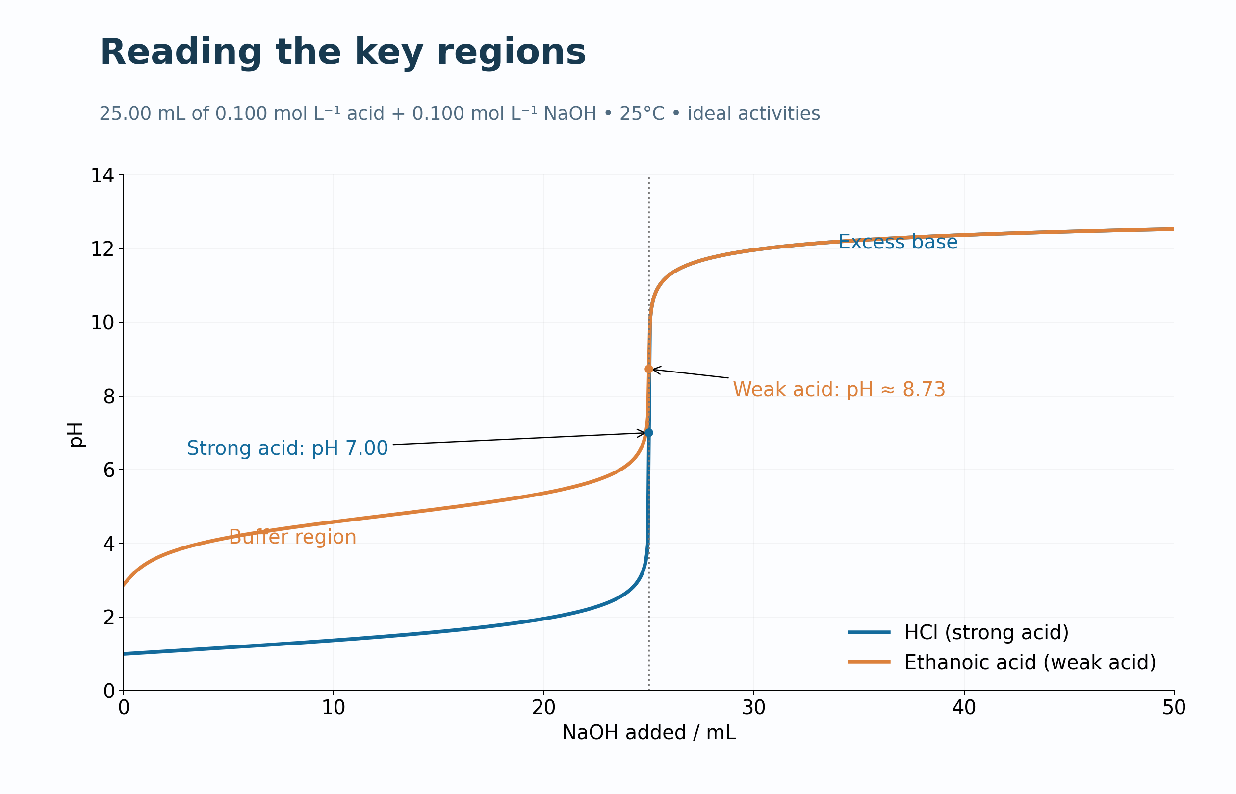
Read the key regions
Annotations identify the buffer region, equivalence points and excess-base region.
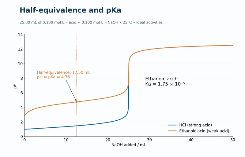
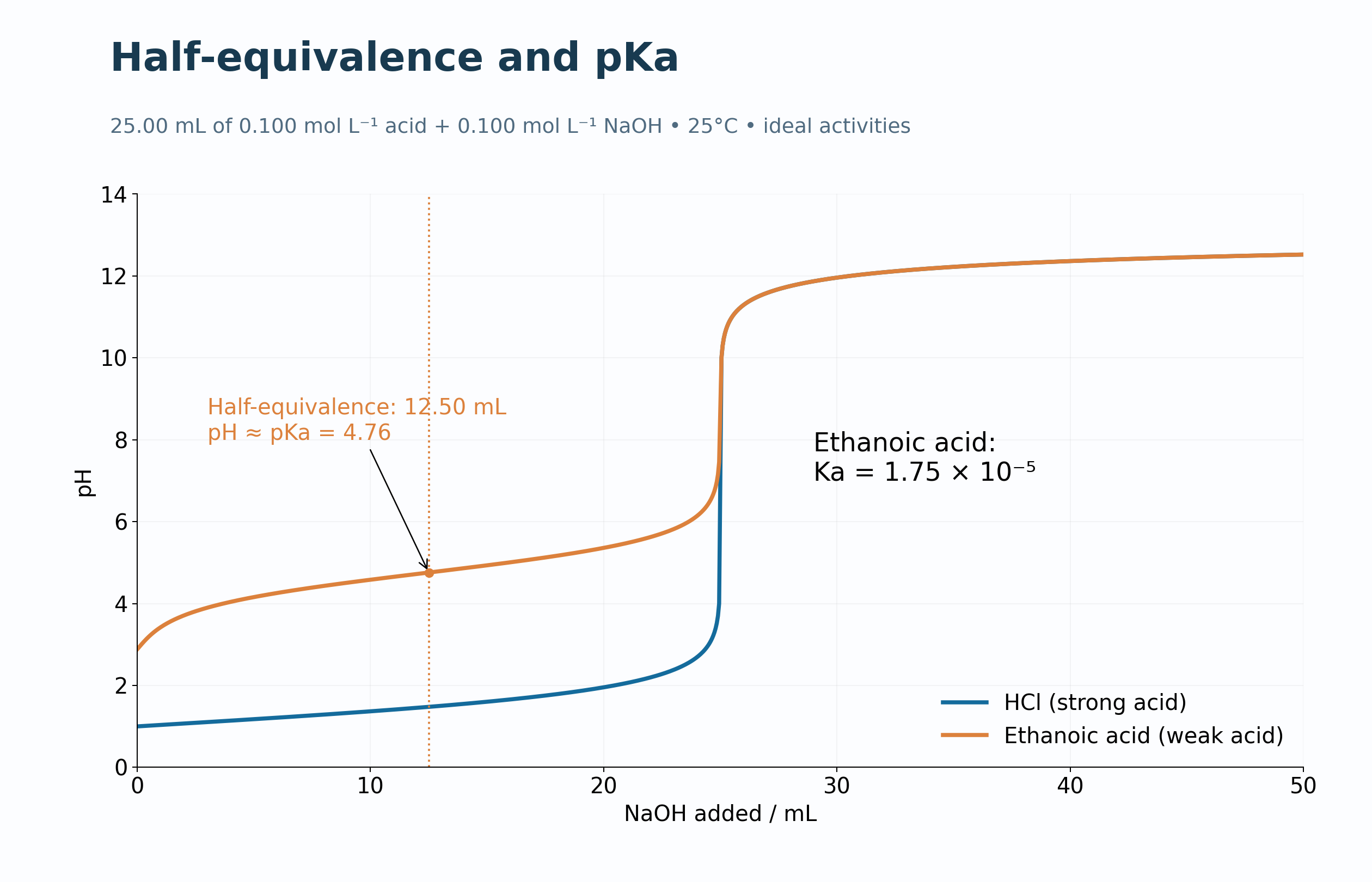
Half-equivalence and pKa
The weak-acid curve highlights half-equivalence at 12.50 mL and pH approximately equal to pKa.
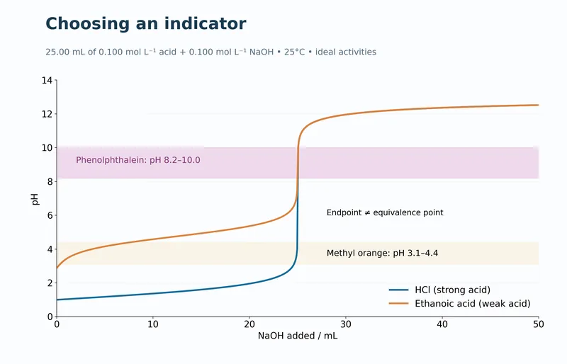
Choose an indicator
Phenolphthalein and methyl-orange transition ranges are compared with the model titration curves.
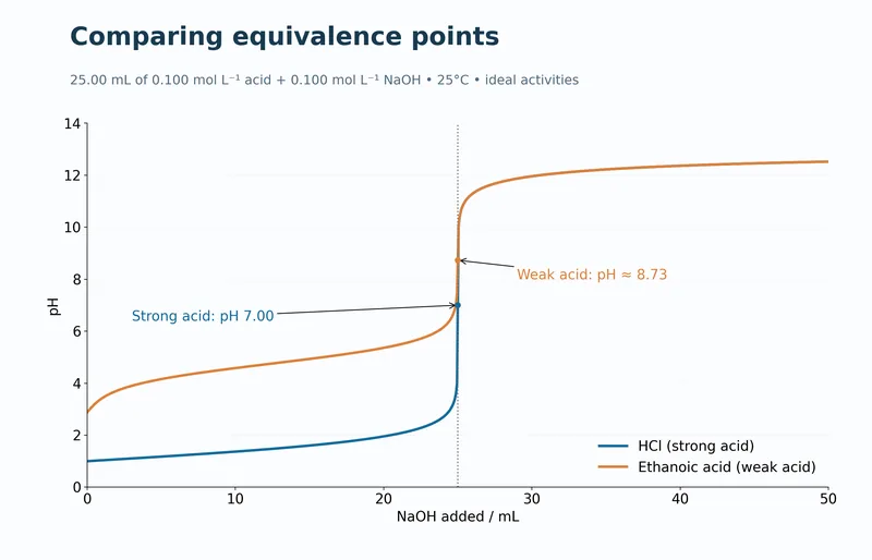
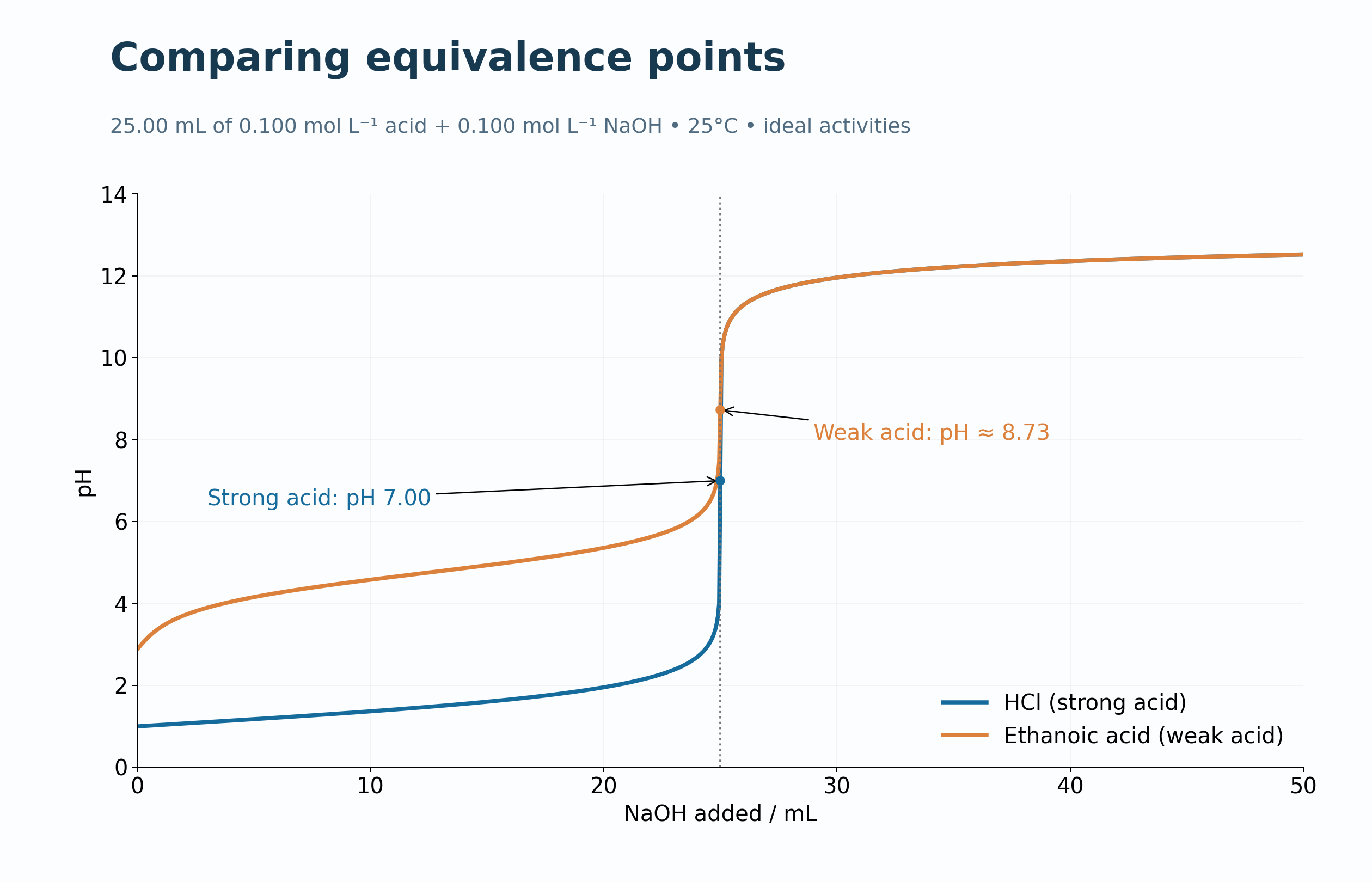
Compare equivalence points
Strong- and weak-acid curves mark equivalence pH values near 7.00 and 8.73.
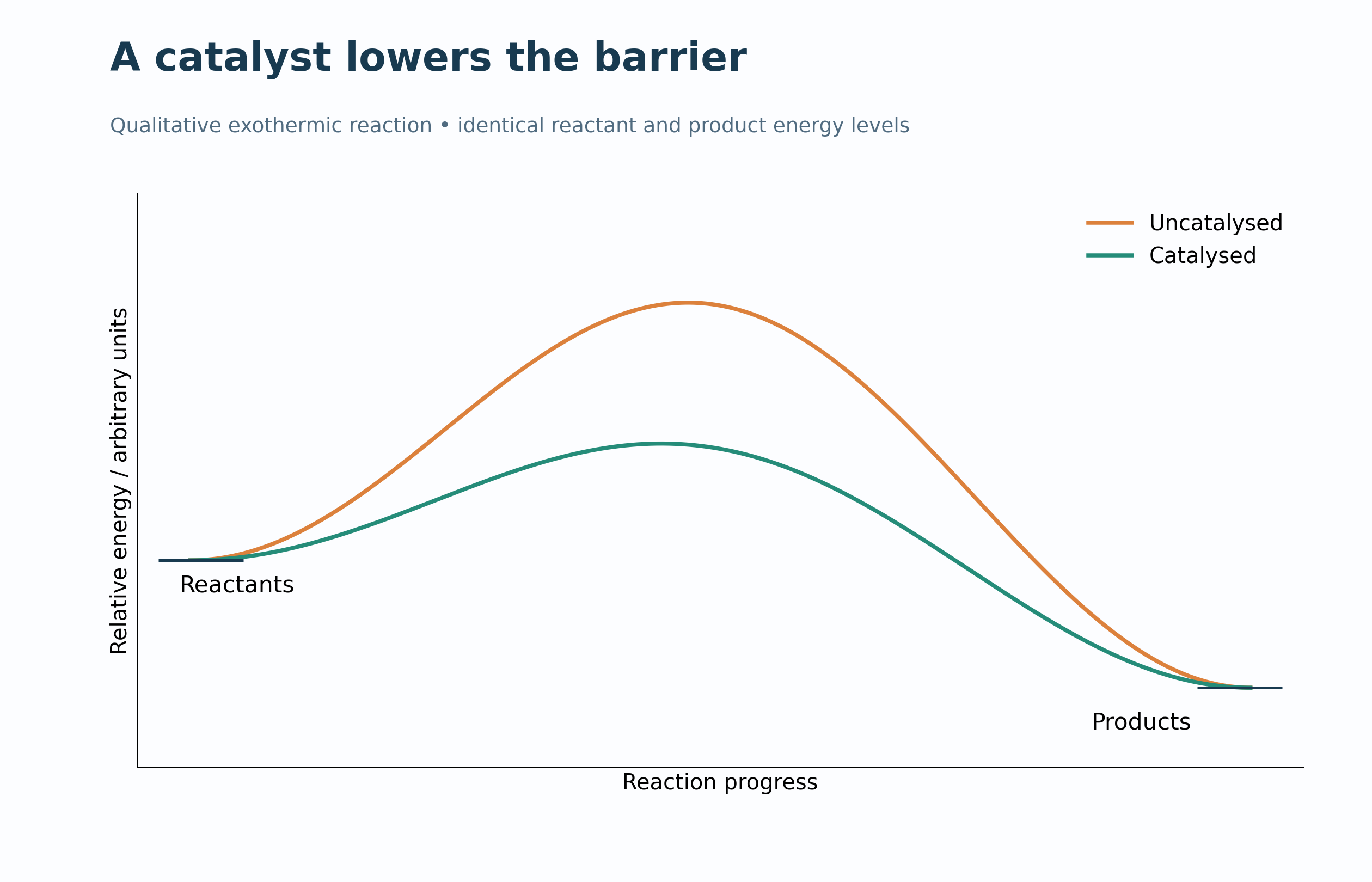
 CHEMISTRY · 5 VISUALSCatalysed and uncatalysed reaction profilesCompare catalysed and uncatalysed pathways without changing reactant or product energy levels.
A lower barrier
Qualitative exothermic profiles compare catalysed and uncatalysed routes.

The same enthalpy change
Activation-energy arrows differ while reactant-to-product enthalpy change remains the same.

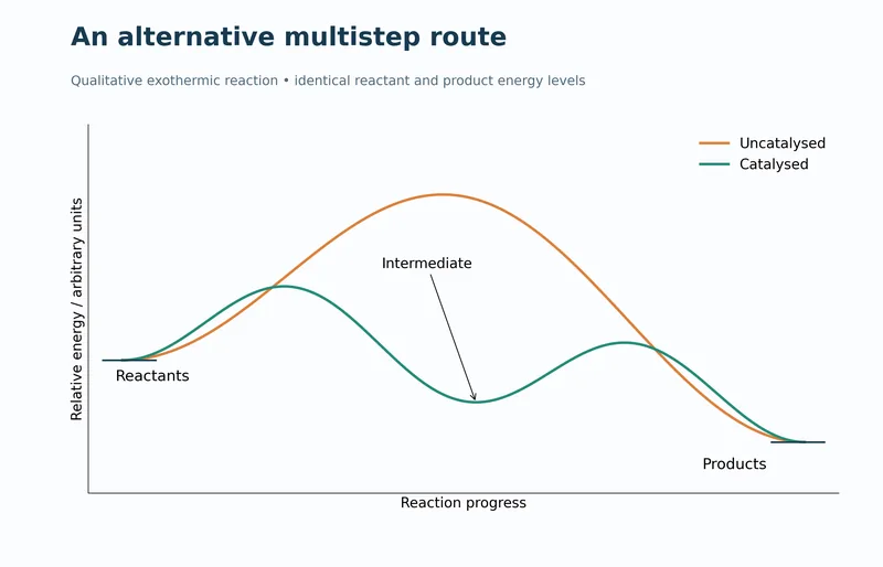
A multistep alternative
A two-step catalysed pathway contains an intermediate between two transition-state peaks.
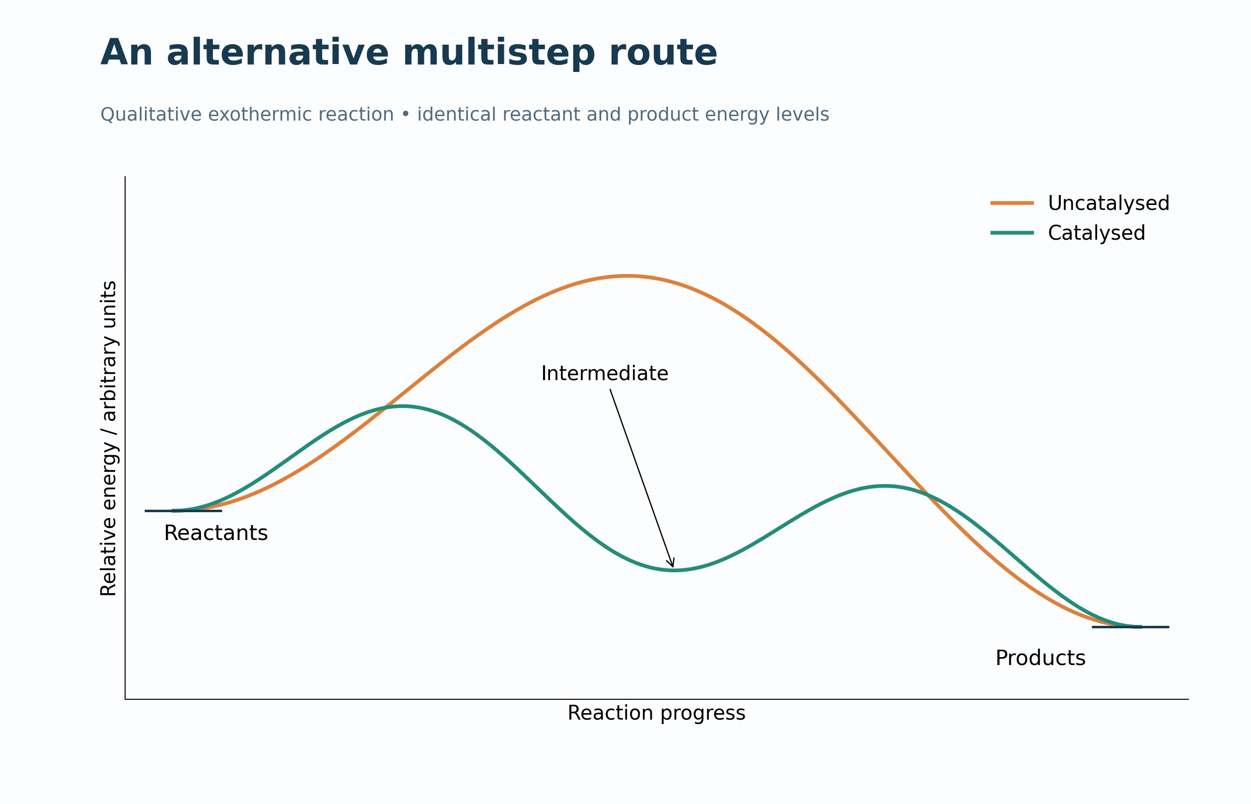
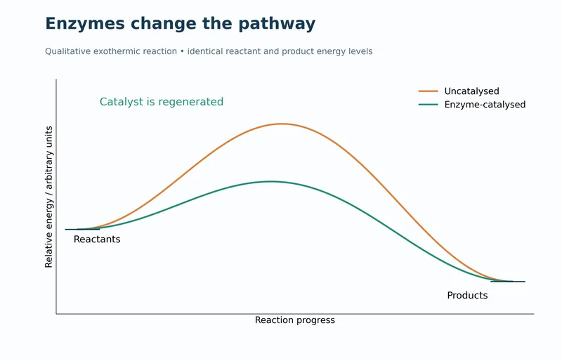
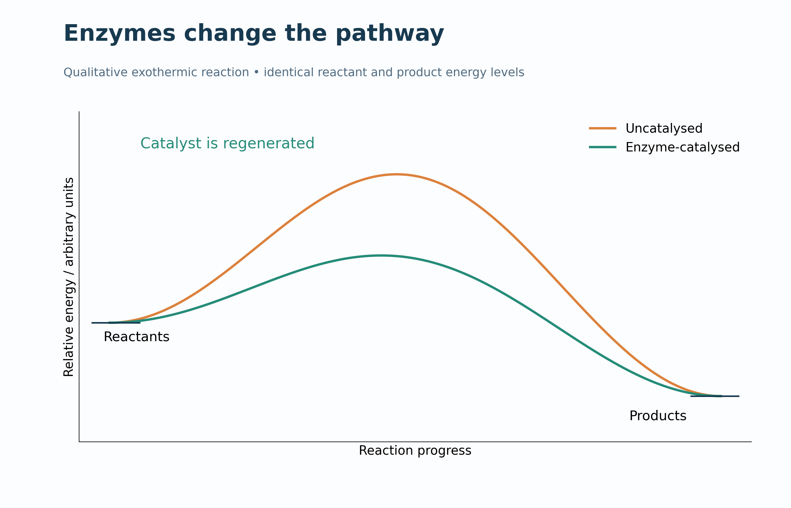
Enzymes change the pathway
A qualitative enzyme-catalysed profile illustrates a lower barrier and catalyst regeneration.
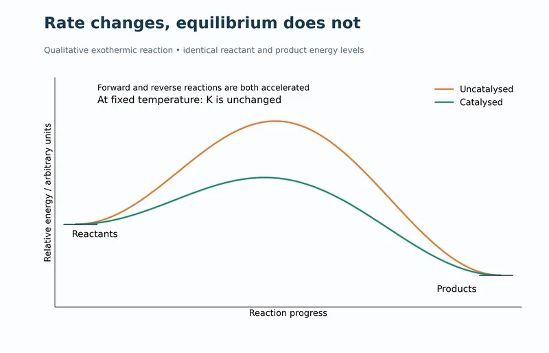
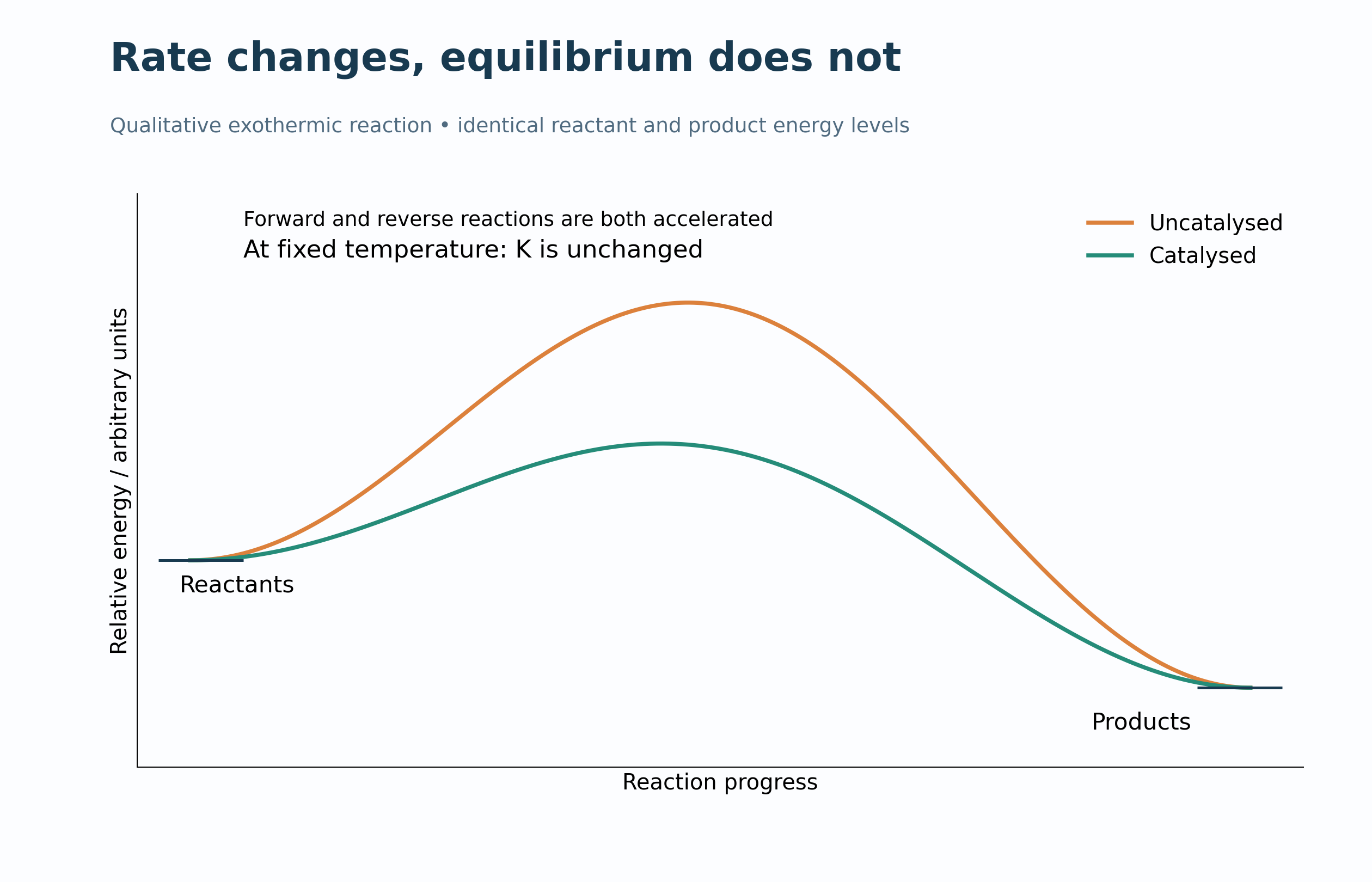
Rate changes, equilibrium does not
Profiles explain faster forward and reverse reactions without changing the equilibrium constant at fixed temperature.
 CHEMISTRY · 5 VISUALSTemperature and the Maxwell–Boltzmann distributionExplore how temperature changes a molecular-energy distribution and the fraction above a chosen threshold.
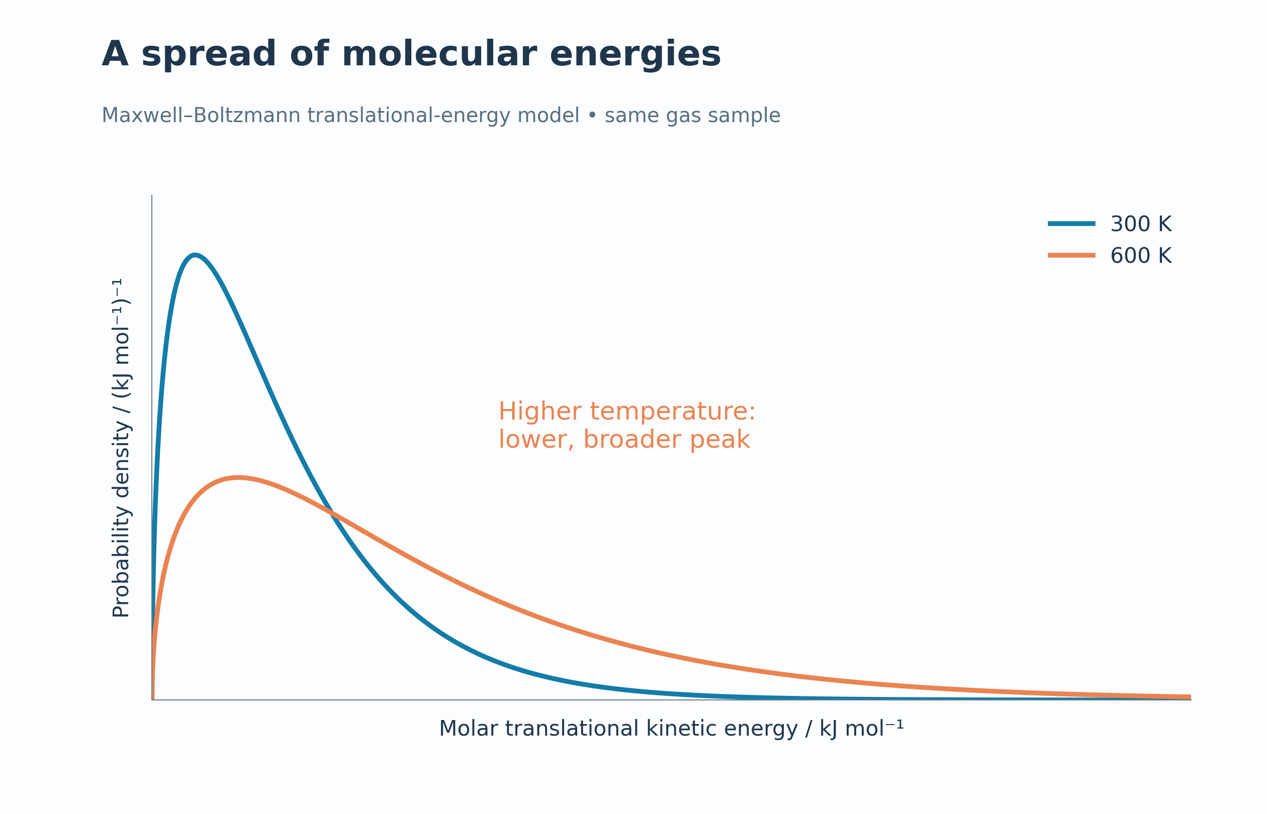
A spread of energies
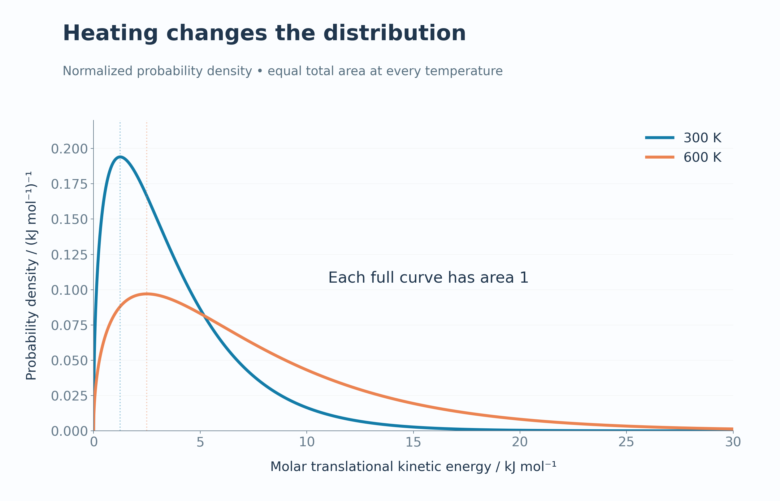
Model distributions at 300 K and 600 K show a lower, broader peak at higher temperature.

Equal total area
Normalised energy-probability curves each have a total area of one.

A fixed threshold
A 12 kJ mol−1 illustrative threshold highlights the high-energy tail at two temperatures.


Heating versus catalysis
A fixed-temperature curve distinguishes lowering a barrier from changing the energy distribution.


Quantify the high-energy tail
Model fractions above 12 kJ mol−1 compare 2.21% at 300 K with 18.62% at 600 K.

 CHEMISTRY · 5 VISUALSHeating curve and changes of stateConnect the regions of a heating curve with warming and changes of state.
Heating a pure substance
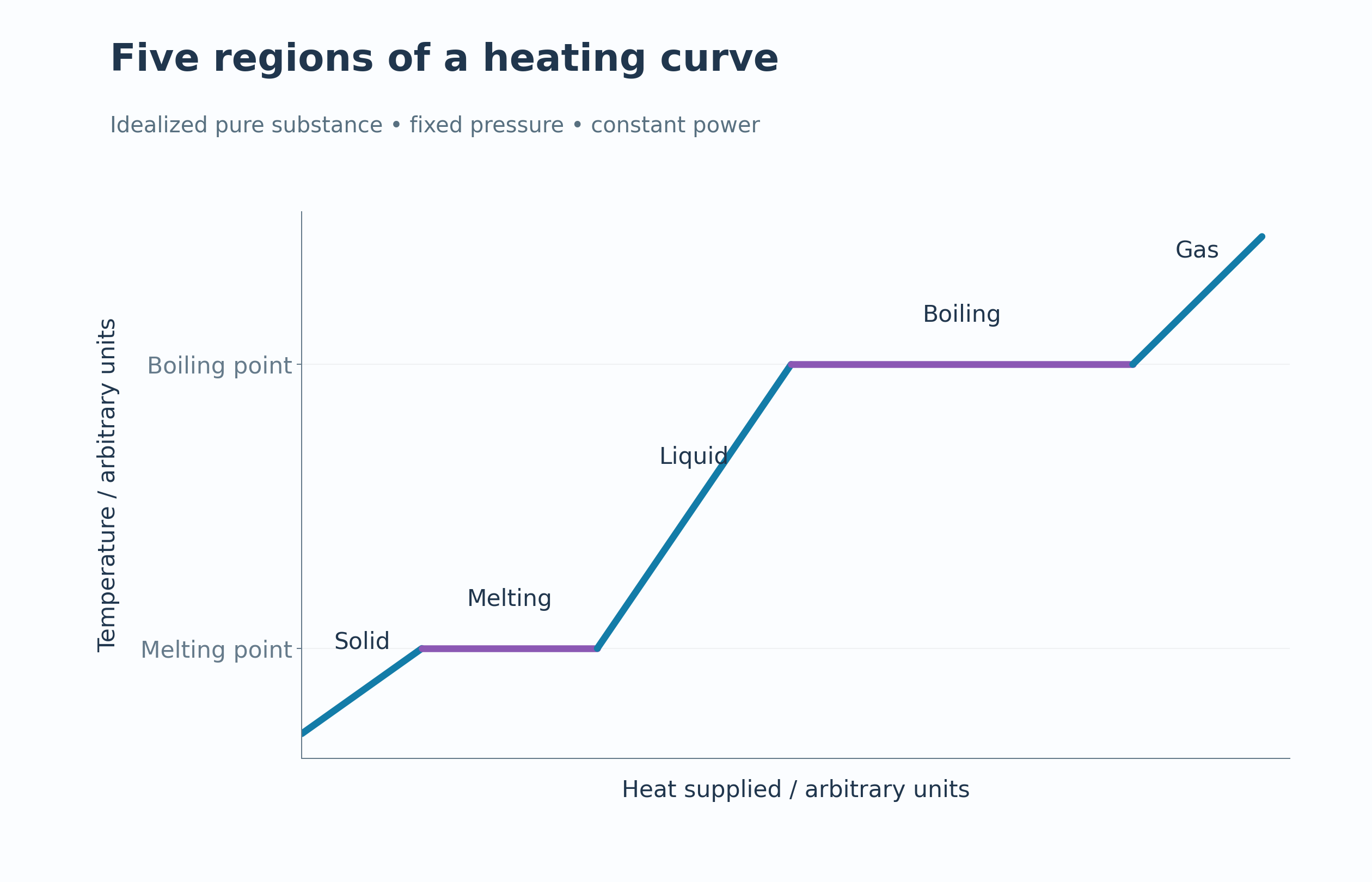
An idealised curve shows warming separated by melting and boiling plateaus.


Five regions
Labels identify solid warming, melting, liquid warming, boiling and gas warming.

Where the energy goes
Slopes use q = mcΔT while phase-change plateaus use q = mL.


Particles across phases
Symbolic particle arrangements accompany the solid, liquid and gas regions.


Heating and cooling
Opposing curves compare heating and cooling with equal power magnitudes.

 CHEMISTRY · 5 VISUALSHydration of ions during dissolvingFollow water orientation around dissolved ions and connect hydration with dissolving and saturation.
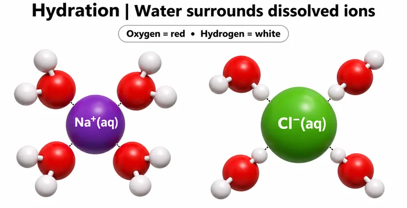
Water surrounds ions
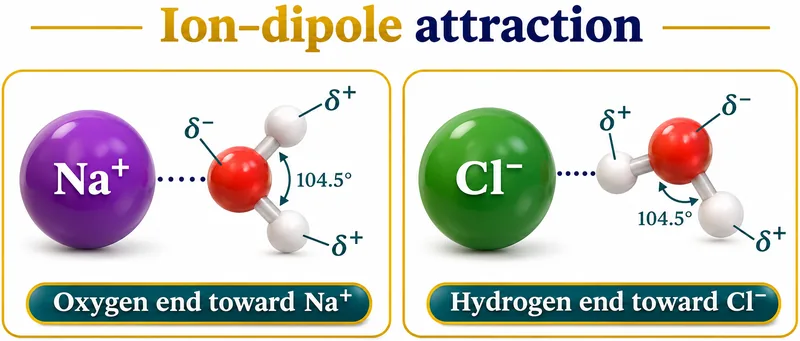
Water molecules face sodium with their oxygen ends and chloride with their hydrogen ends.

Ion–dipole attraction
Partial charges explain the orientation of water near a cation or an anion.


Ions leave the lattice
An illustrative salt surface shows ions separating and becoming hydrated in water.


Energy contributions
A qualitative endothermic cycle combines lattice dissociation and hydration enthalpies.


A dynamic balance
A saturated solution in contact with solid has equal dissolving and crystallising rates at equilibrium.

 CHEMISTRY · 5 VISUALSDiamond, graphite and grapheneRelate diamond, graphite and graphene bonding networks to their properties.
Two architectures
Idealised fragments contrast diamond’s three-dimensional network with graphite’s stacked sheets.
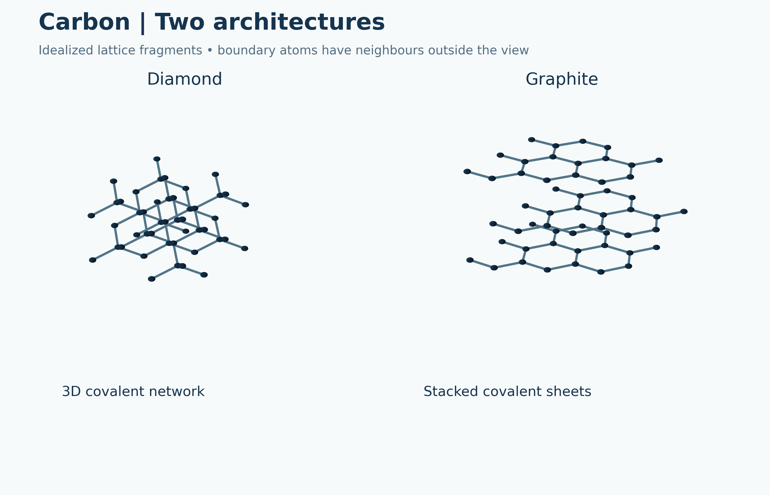

Bonding networks
Diamond’s four neighbours per bulk atom are compared with three neighbours per graphite-sheet atom.


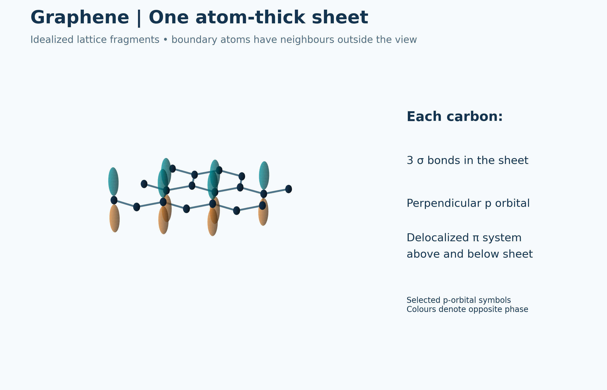
One atom-thick sheet
A graphene fragment shows in-plane sigma bonding and symbolic perpendicular p orbitals.

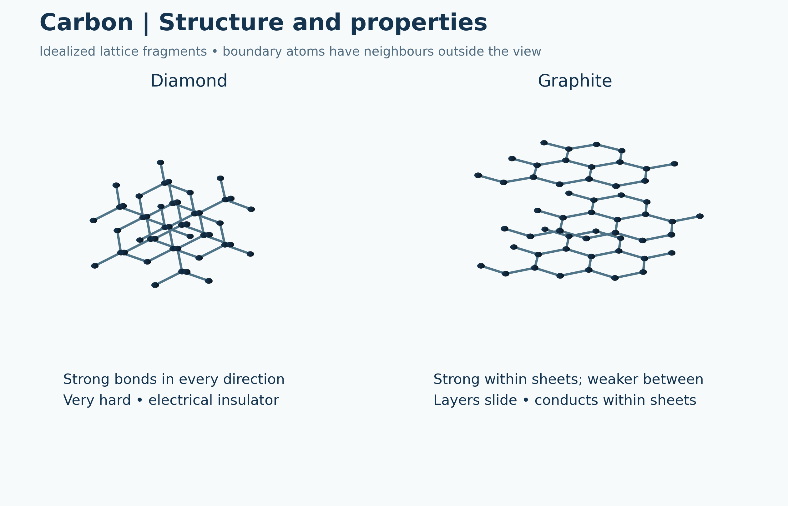
Structure and properties
Network differences are connected with hardness, sliding layers and electrical conduction.

Three related structures
Side-by-side lattice fragments compare diamond, graphite and graphene.

 CHEMISTRY · 5 VISUALSSigma and pi bonding in etheneConnect ethene’s planar structure with sigma bonding, pi overlap and restricted rotation.
A planar double bond
An ethene formula shows the planar framework, approximate bond angles and sigma/pi bond count.
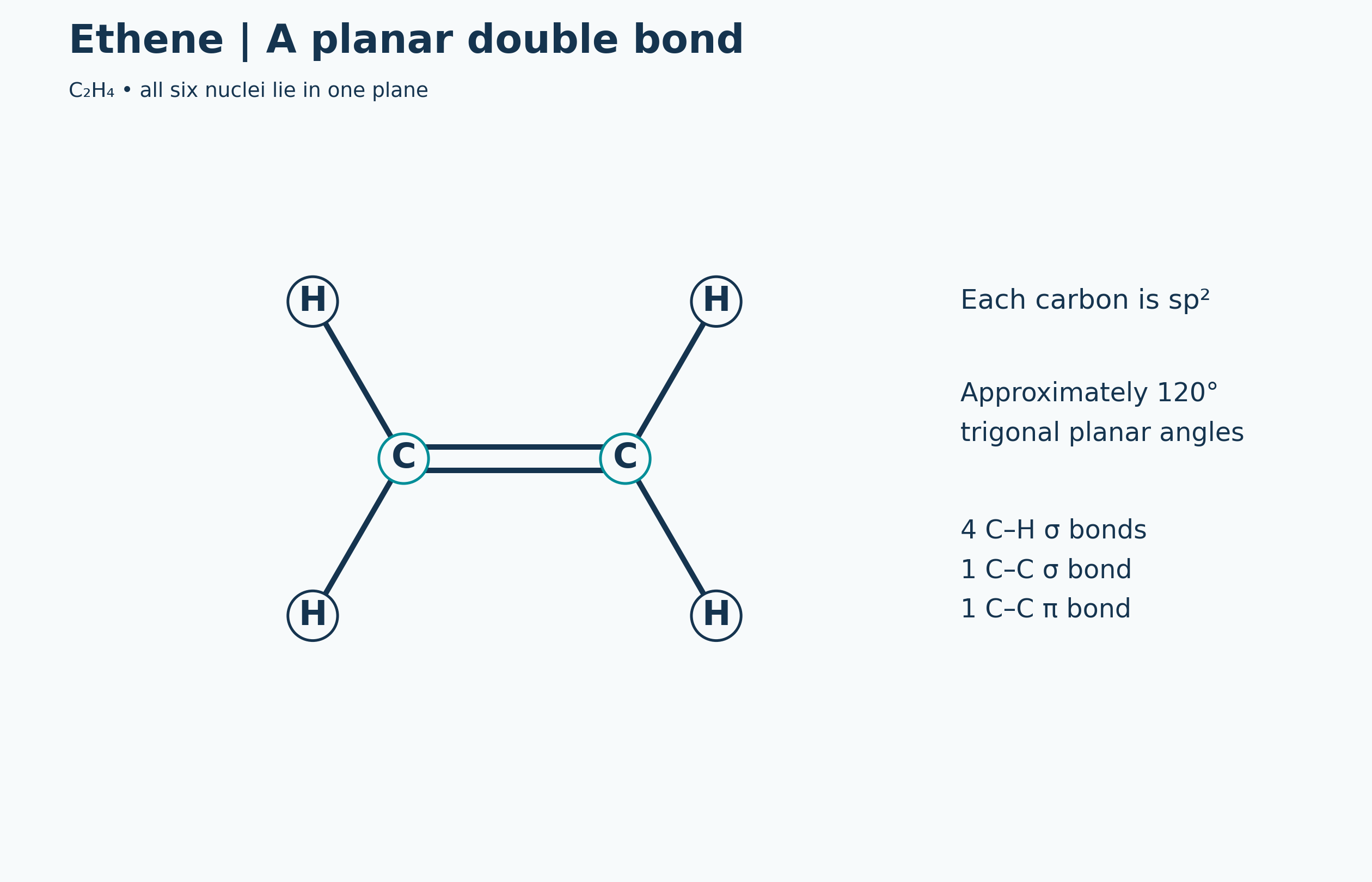

One sigma and one pi bond
The molecular-plane sigma framework is compared with pi overlap above and below the plane.

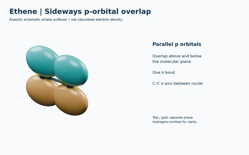
Sideways p-orbital overlap
Conceptual phase surfaces illustrate parallel p orbitals forming one pi bond.

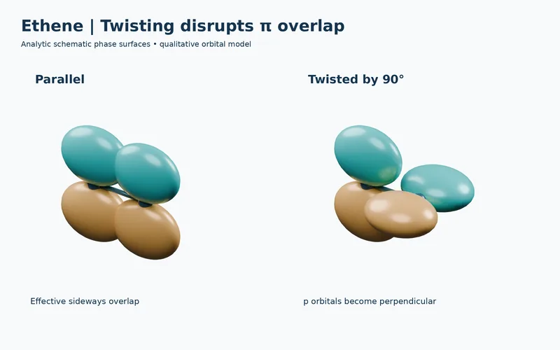
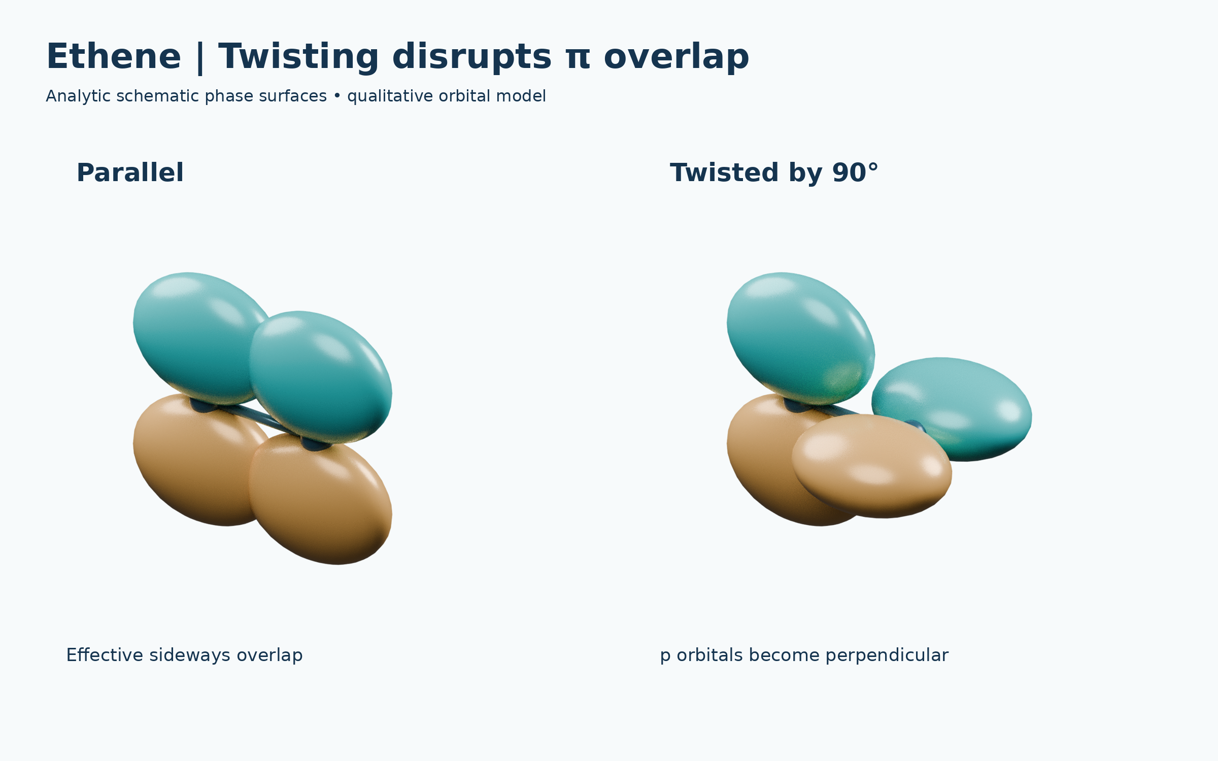
Twisting disrupts overlap
Parallel and 90°-twisted orbital models compare effective and disrupted sideways overlap.
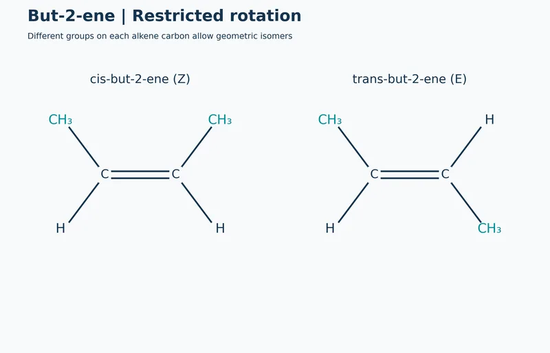
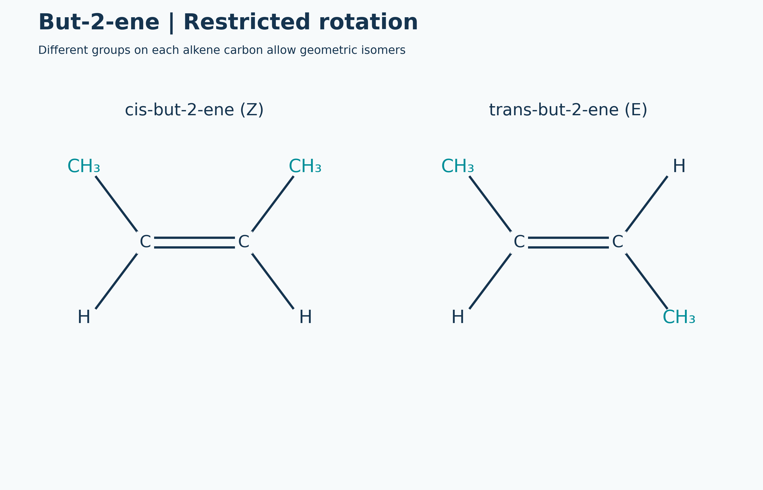
Restricted rotation and isomers
Cis and trans but-2-ene formulae connect restricted rotation with geometric isomerism.
 CHEMISTRY · 5 VISUALSNuclide notation and isotopesRead nuclide notation and distinguish isotope changes from electron loss and relative atomic mass.
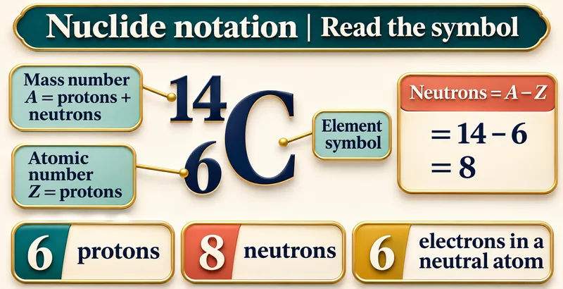
Read the symbol
Carbon-14 notation identifies mass number, atomic number and the resulting particle counts.


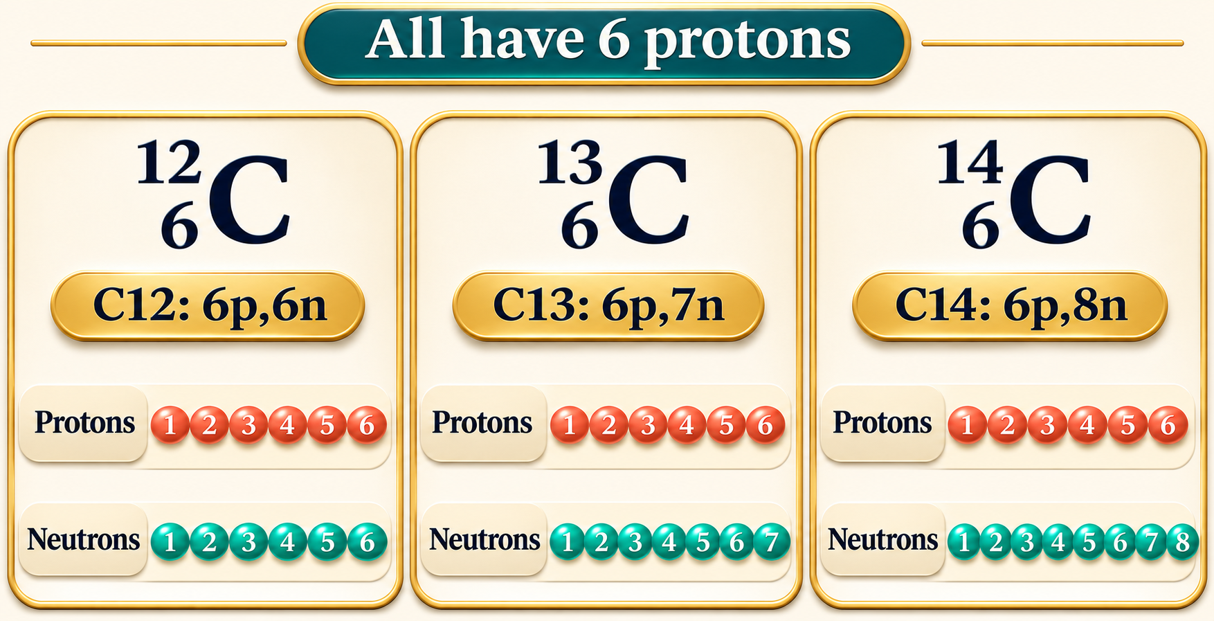
All have six protons
Carbon-12, carbon-13 and carbon-14 share six protons but differ in neutron number.
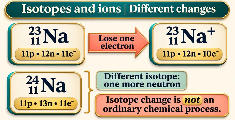
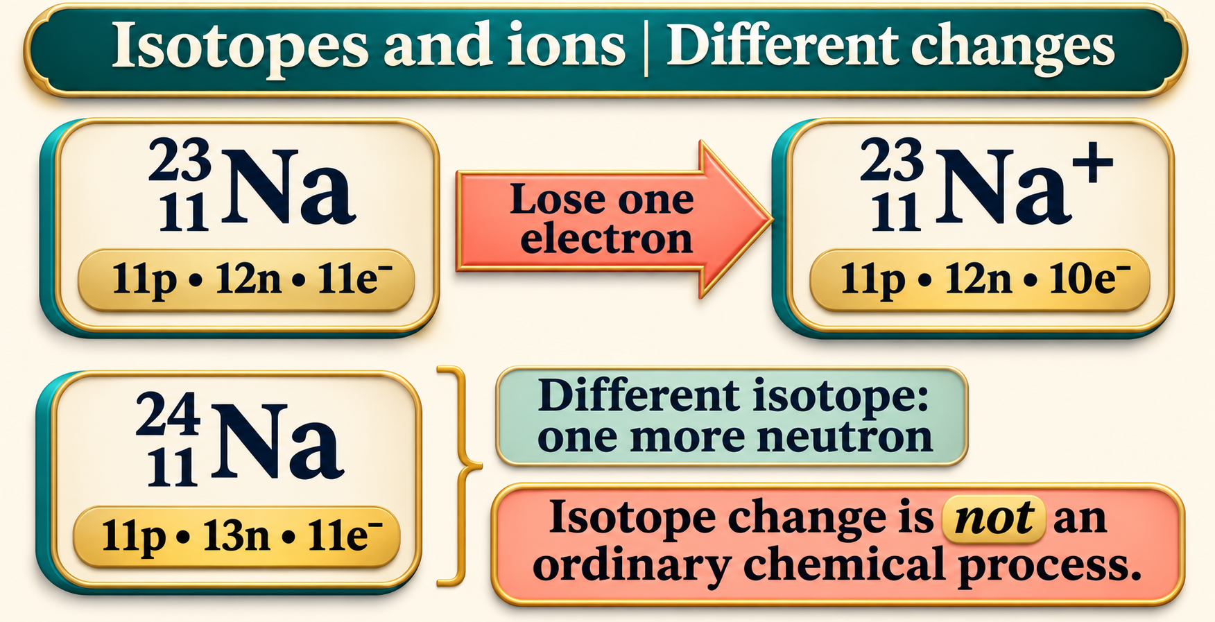
Isotopes and ions
Sodium examples distinguish losing an electron from changing the number of neutrons.

Mass number versus relative atomic mass
A whole-number nuclear count is contrasted with the weighted relative atomic mass of an element.


Balance alpha decay
Uranium-238 alpha decay conserves total mass number and atomic number.

 CHEMISTRY · 5 VISUALSReading an isotope mass spectrumInterpret chlorine isotope peaks and calculate approximate atomic and molecular isotope patterns.
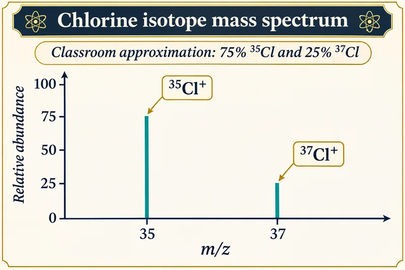
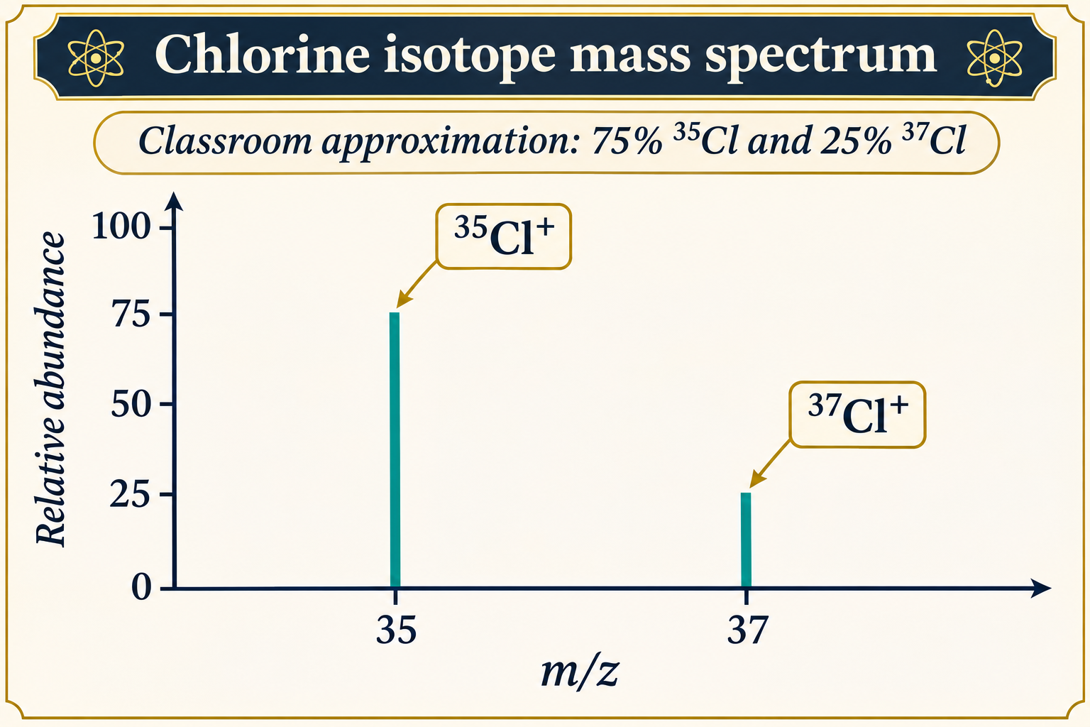
Chlorine isotope peaks
An illustrative chlorine-ion spectrum uses approximate 75% chlorine-35 and 25% chlorine-37 abundances.

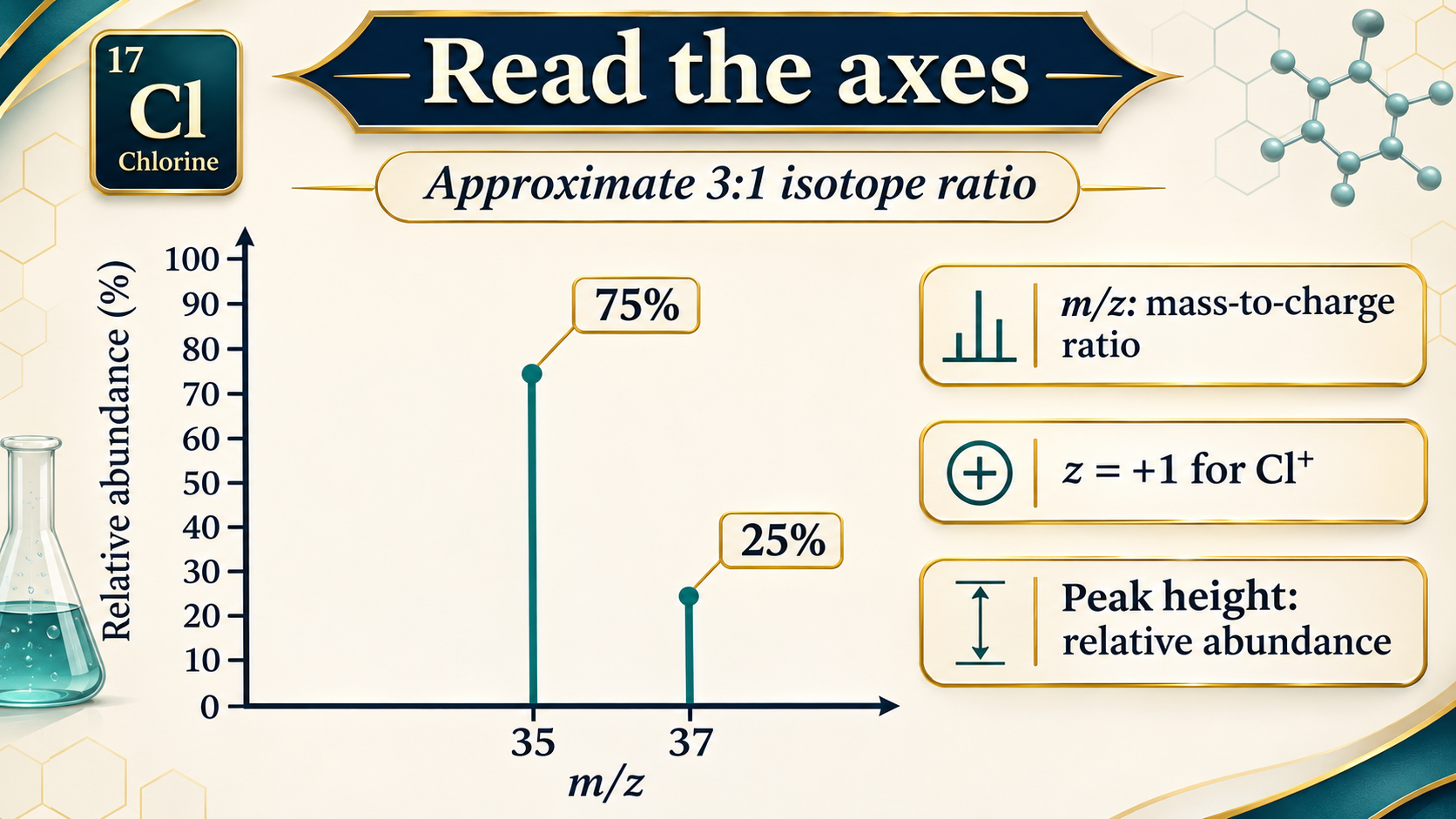
Read the axes
Labels explain mass-to-charge ratio and relative abundance for singly charged chlorine ions.
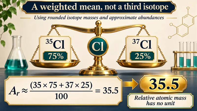
A weighted mean
A classroom calculation uses rounded masses and abundances to obtain relative atomic mass about 35.5.
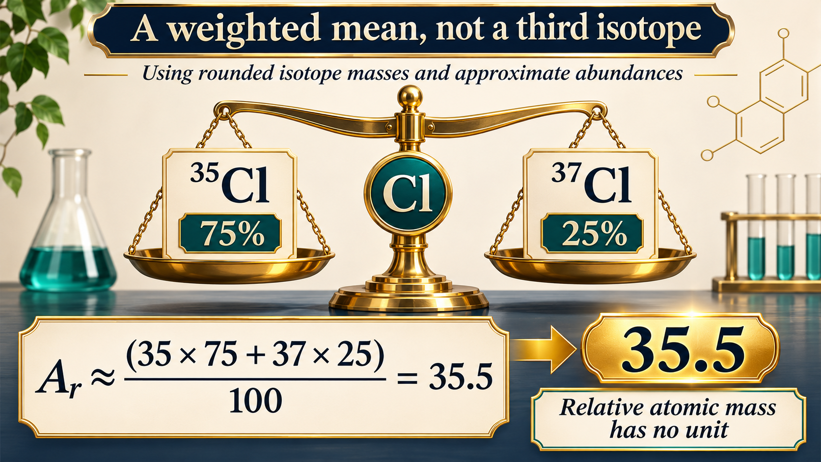
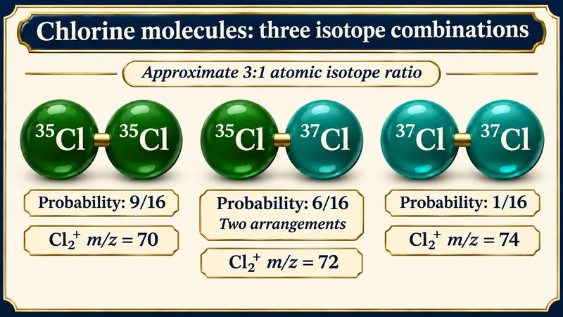
Three isotope combinations
Chlorine molecules give approximate probabilities 9/16, 6/16 and 1/16 for the three mass combinations.
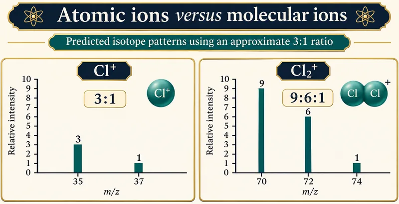
Atomic versus molecular ions
Predicted Cl+ and Cl2+ isotope patterns compare approximate 3:1 and 9:6:1 intensity ratios.

 CHEMISTRY · 5 VISUALSIonic and covalent bonding with electron diagramsUse outer-electron diagrams to compare ionic transfer, covalent sharing and a donated electron pair.
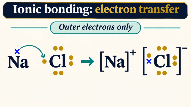
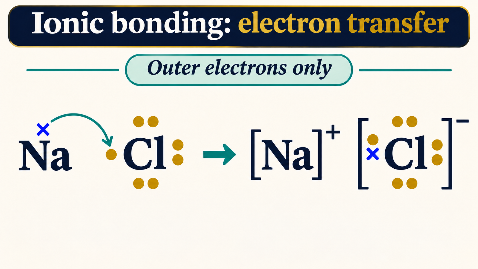
Electron transfer
Outer-electron diagrams show sodium transferring an electron and forming Na+ and Cl−.

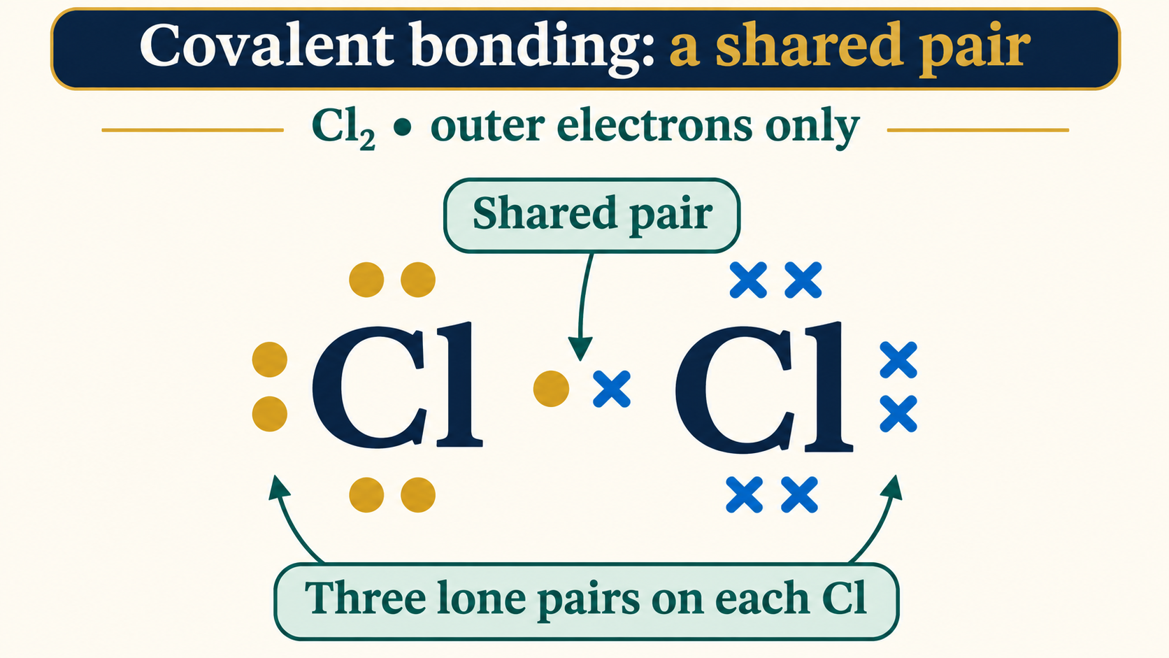
A shared pair
A chlorine molecule has one shared electron pair and three lone pairs on each atom.

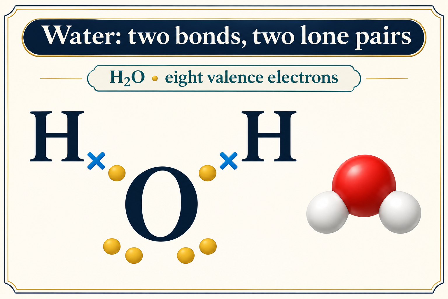
Water’s valence electrons
A water diagram shows two bonding pairs and two lone pairs around oxygen.

A donated pair
Ammonia donates a lone pair to H+ to form ammonium with four equivalent N–H bonds.


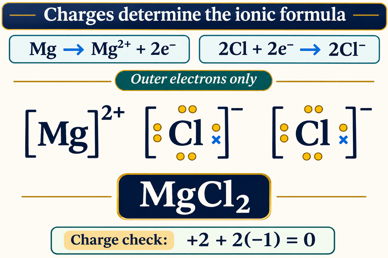
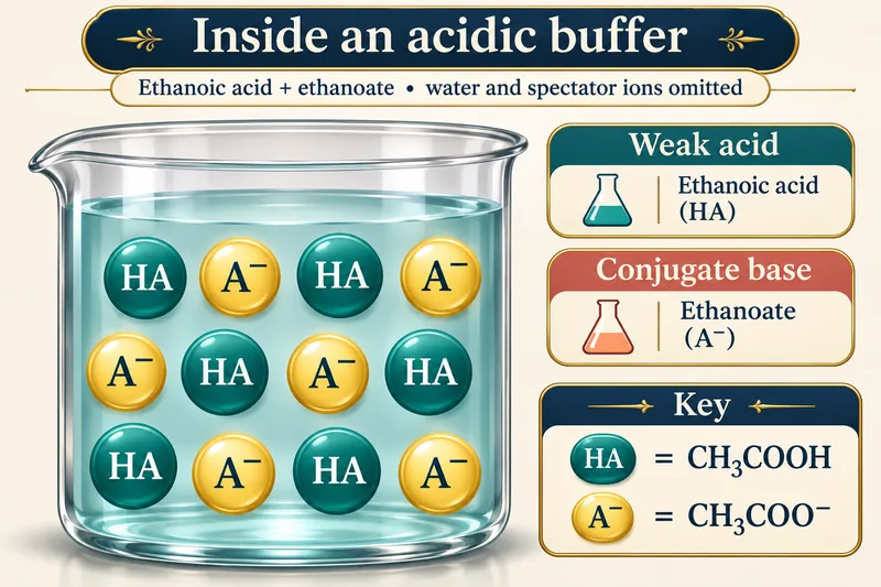
Charges determine the formula
Magnesium and chloride electron diagrams support MgCl2 and a zero total charge.
 CHEMISTRY · 5 VISUALSHow a buffer resists pH changeExplain how a weak acid and its conjugate base resist small additions of acid or base.
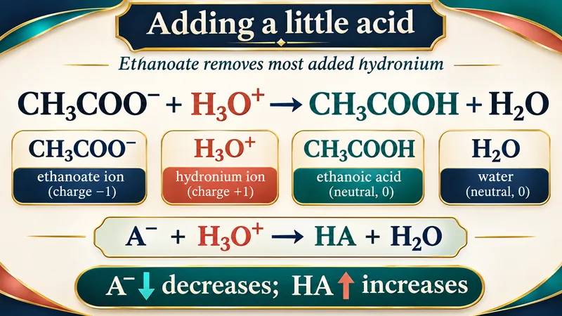
Inside an acidic buffer
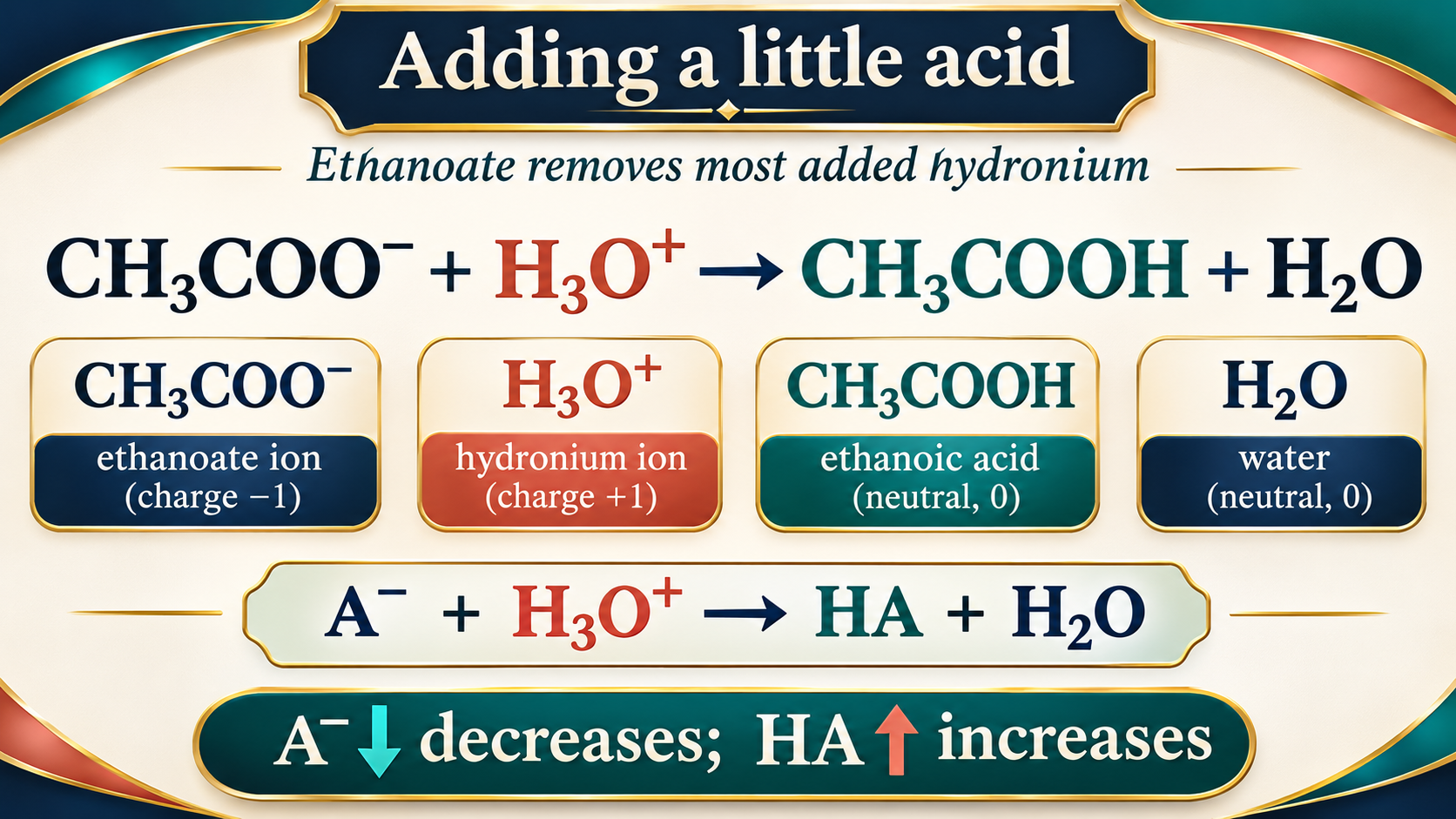
Ethanoic acid and ethanoate are represented as the weak-acid and conjugate-base components.

Adding acid
Ethanoate reacts with added hydronium, increasing ethanoic acid and reducing conjugate base.
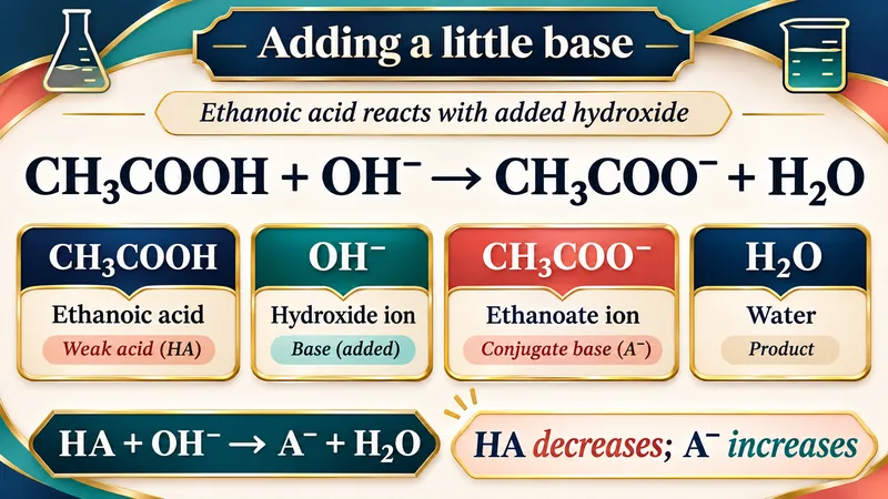
Adding base
Ethanoic acid reacts with hydroxide to form ethanoate and water.


The acid–base ratio
The Henderson–Hasselbalch approximation relates pH to pKa and the conjugate-base/acid concentration ratio.


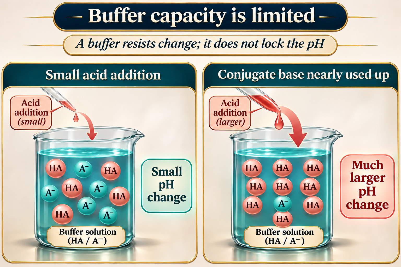
Capacity is limited
A comparison shows a small pH change for a small acid addition and a larger change as conjugate base is depleted.
 CHEMISTRY · 5 VISUALSDynamic equilibriumDistinguish equal forward and reverse rates from equal concentrations at dynamic equilibrium.
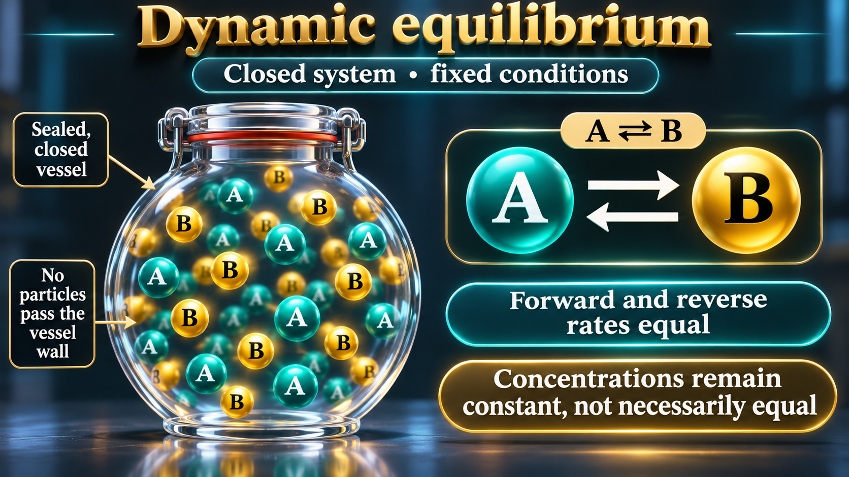
A closed system
A sealed-vessel model shows continuing forward and reverse reactions with constant, not necessarily equal, concentrations.

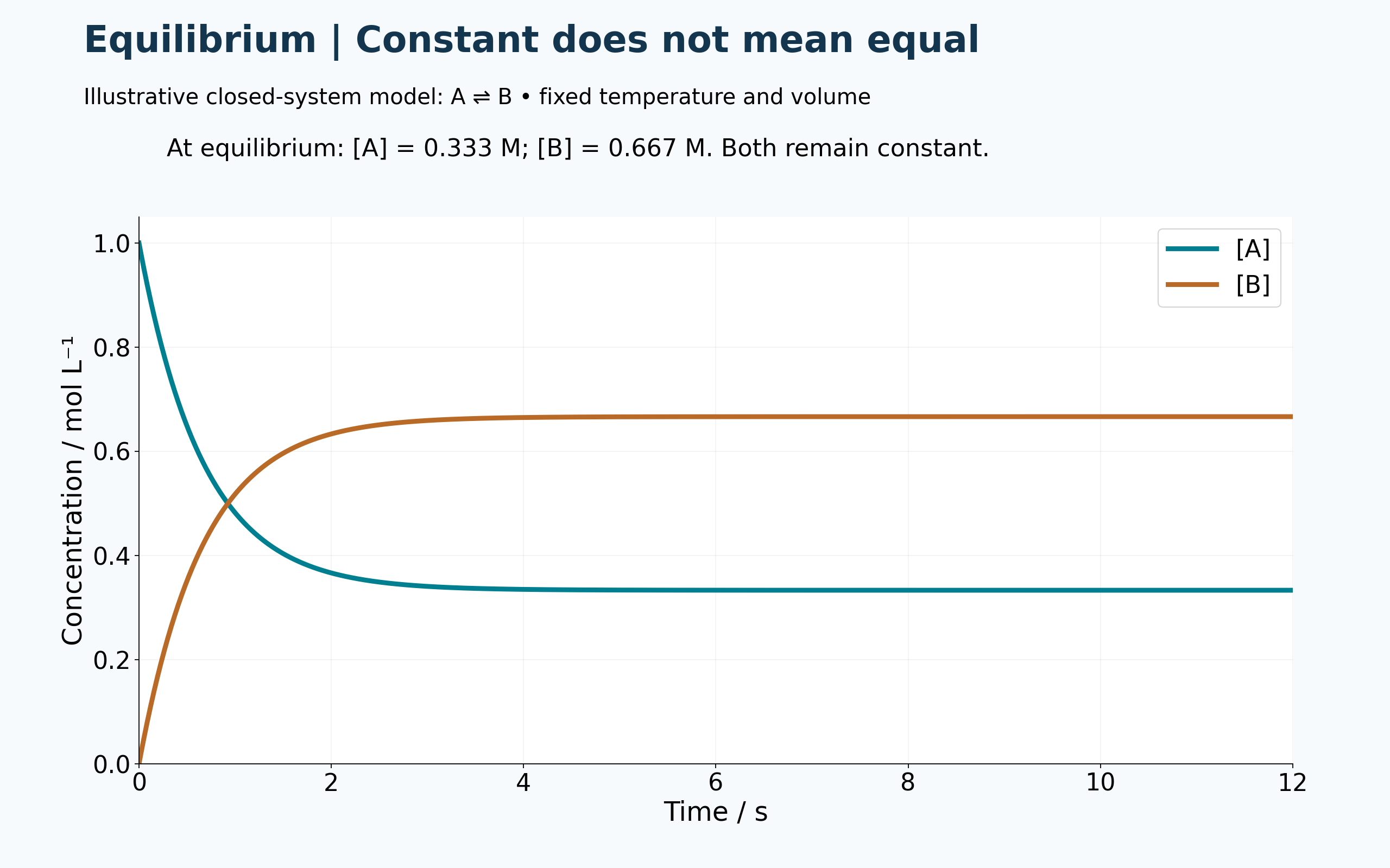
Constant does not mean equal
An illustrative A ⇌ B model reaches unequal but constant concentrations.
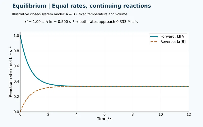
Equal rates
Forward and reverse rates approach the same nonzero value in the model system.

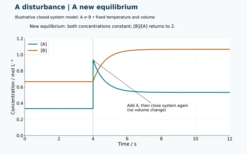
After a disturbance
Adding A produces a new equilibrium while the model equilibrium concentration ratio returns to two.

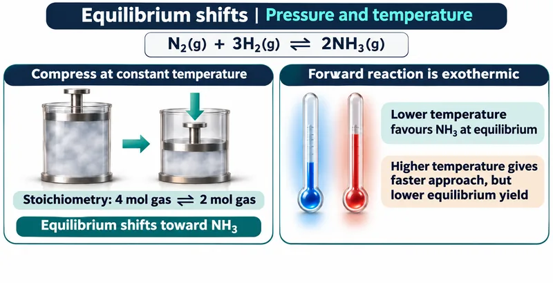
Pressure and temperature
An ammonia-equilibrium comparison separates the effects of compression and temperature on equilibrium and rate.

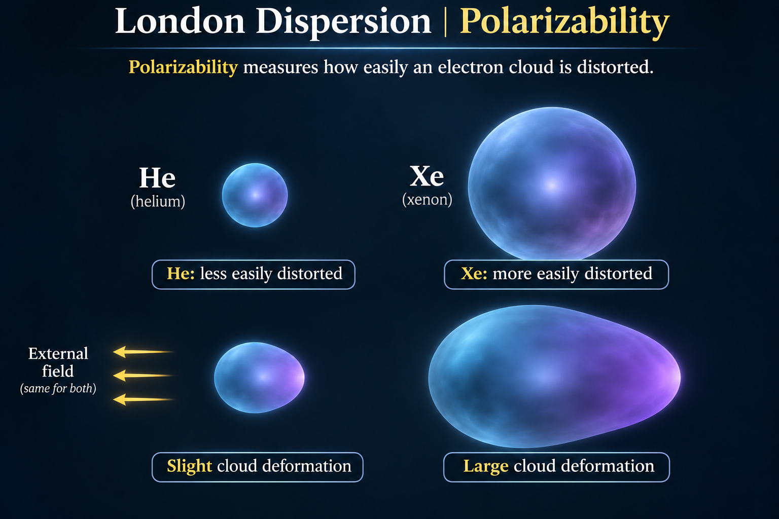
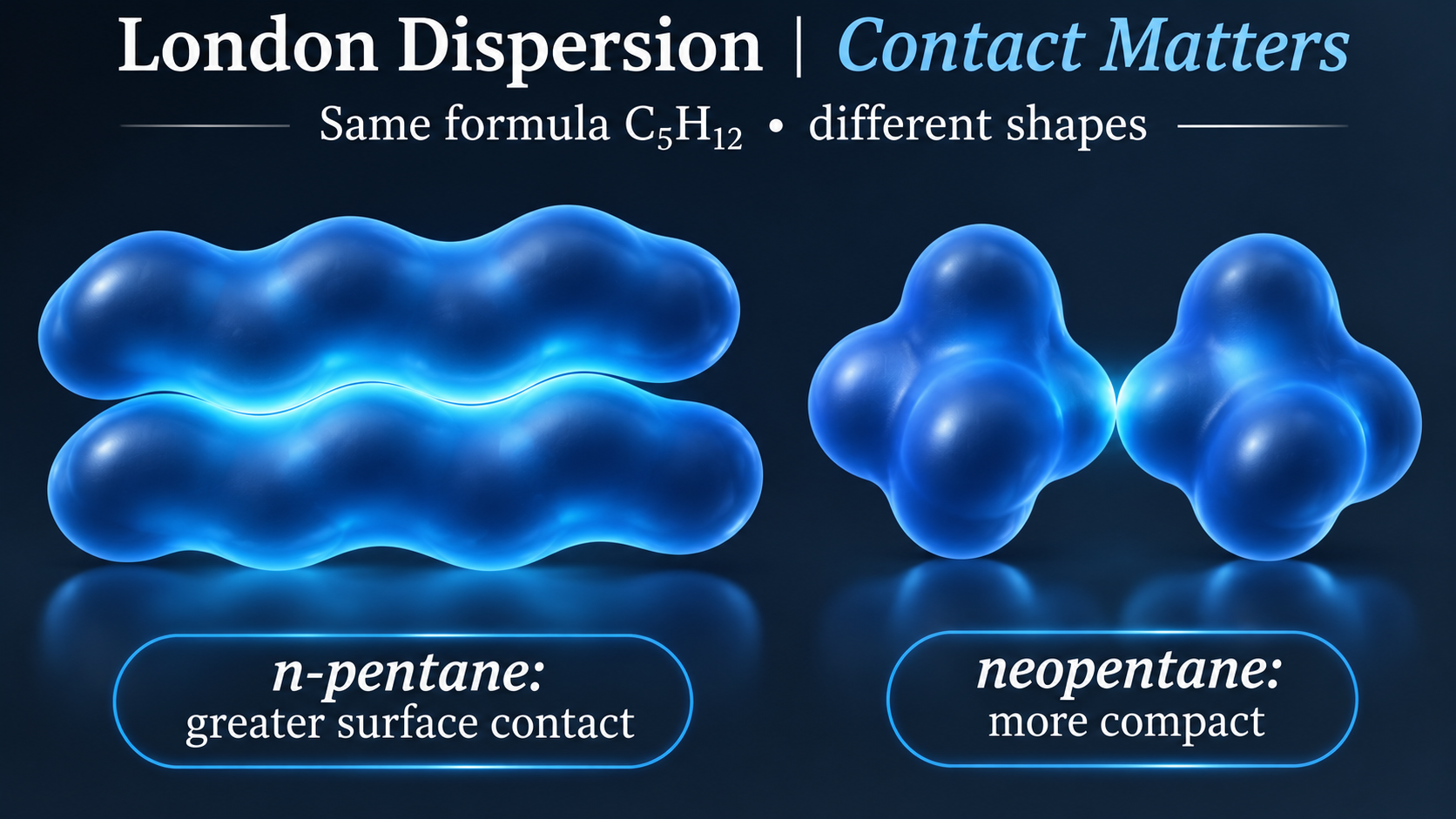
 CHEMISTRY · 5 VISUALSLondon dispersion forcesLondon dispersion comes from correlated fluctuations in electron clouds. These views connect temporary dipoles with polarizability and molecular shape.
Temporary dipoles in argon
Two argon clouds show instantaneous and induced partial charges with an attraction between unlike ends.


Fluctuating electron clouds
Three panels contrast an average symmetric argon cloud with two snapshots of correlated temporary dipoles.


Polarizability: helium and xenon
Helium and xenon clouds respond differently to the same external field, illustrating ease of distortion.

Molecular shape and contact
Qualitative envelopes compare greater contact between elongated n-pentane molecules with compact neopentane.

A molecular view of dispersion
An isolated argon average is compared with two correlated, distorted clouds and their attraction.

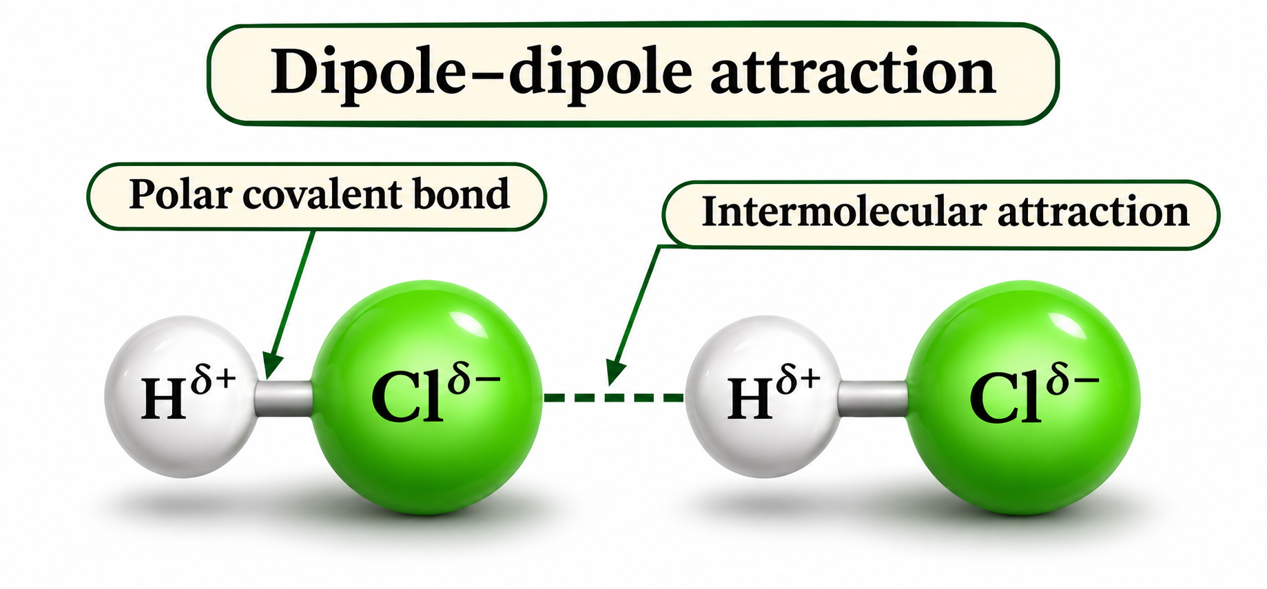
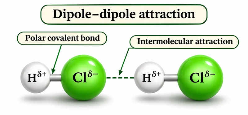 CHEMISTRY · 5 VISUALSDipole–dipole attractionsPermanent dipoles make molecular orientation important. HCl provides a clear example for separating a polar bond from attraction between molecules.
Bond or intermolecular attraction?
Two HCl molecules distinguish the polar covalent H–Cl bond from attraction between neighbouring molecules.

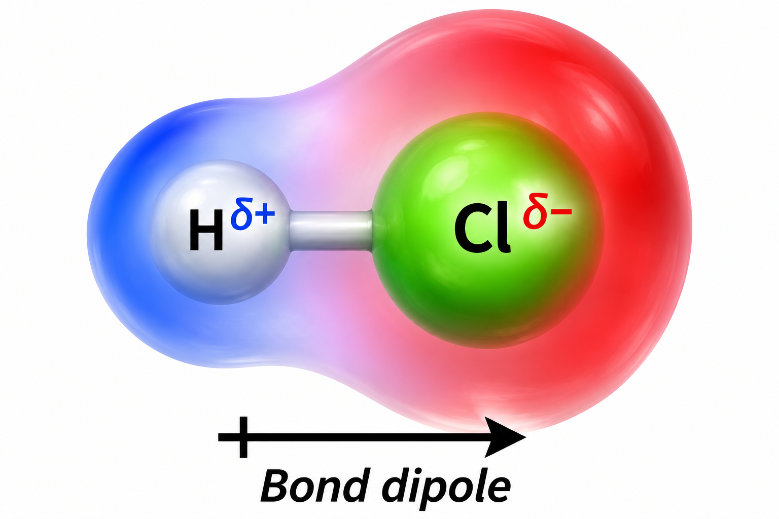
The HCl bond dipole
A coloured HCl envelope and positive-tail arrow show the dipole pointing towards chlorine.
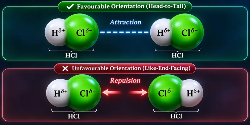
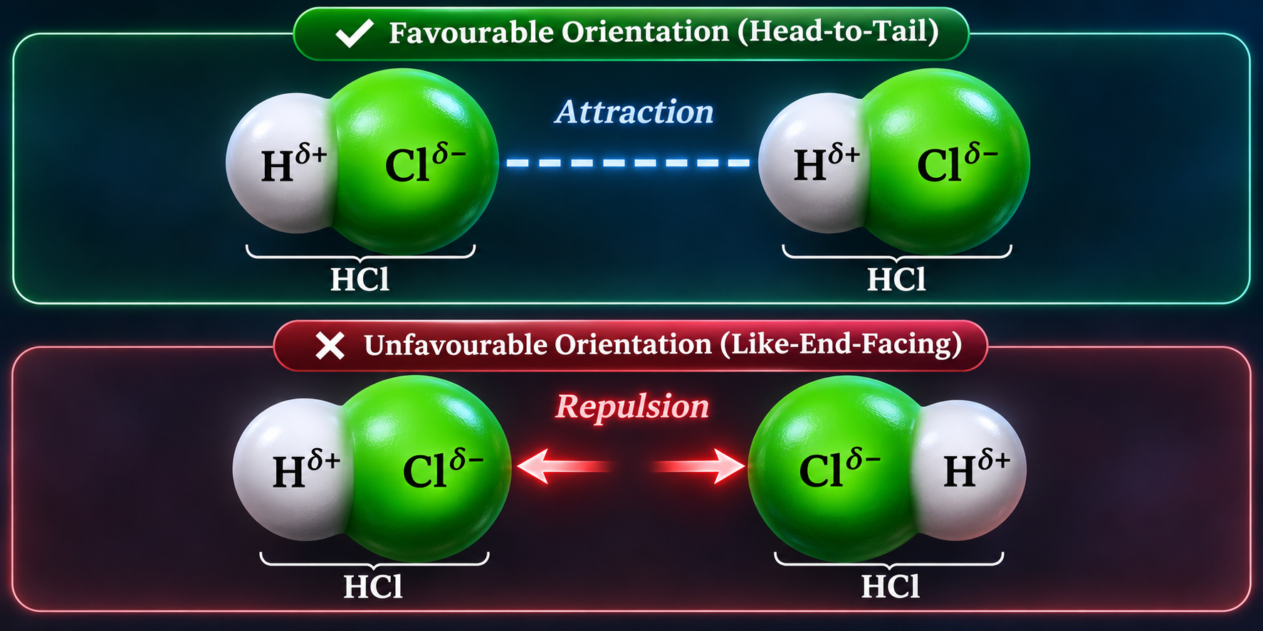
Favourable and unfavourable orientations
Head-to-tail HCl molecules attract; an arrangement with like partial charges facing illustrates repulsion.
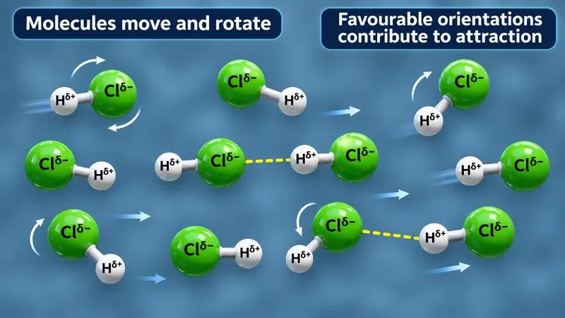
Moving and rotating polar molecules
Several HCl molecules illustrate motion, rotation and favourable attractive orientations.


Nonpolar F2 and polar HCl
F2 has London dispersion; HCl has dispersion and permanent dipole–dipole attractions.

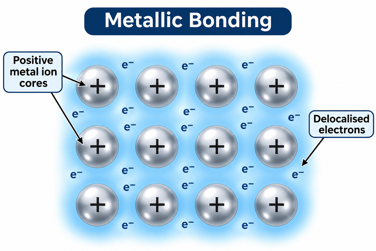
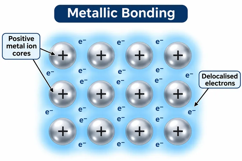 CHEMISTRY · 5 VISUALSMetallic bonding and alloy structureMetallic bonding links positive ion cores with delocalised electrons. The set connects that model with conduction, malleability and alloy strengthening.
The metallic bonding model
Positive metal ion cores sit within a shared region of delocalised electrons.

Electron drift and electric field
Opposite arrows show electron drift against the external electric field through fixed positive cores.


Sliding metal layers
Before-and-after lattice views illustrate layer slip while attraction to delocalised electrons remains.

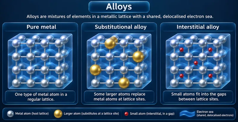
Substitutional and interstitial alloys
Three lattice views compare a pure metal, replacement atoms and small atoms occupying gaps.


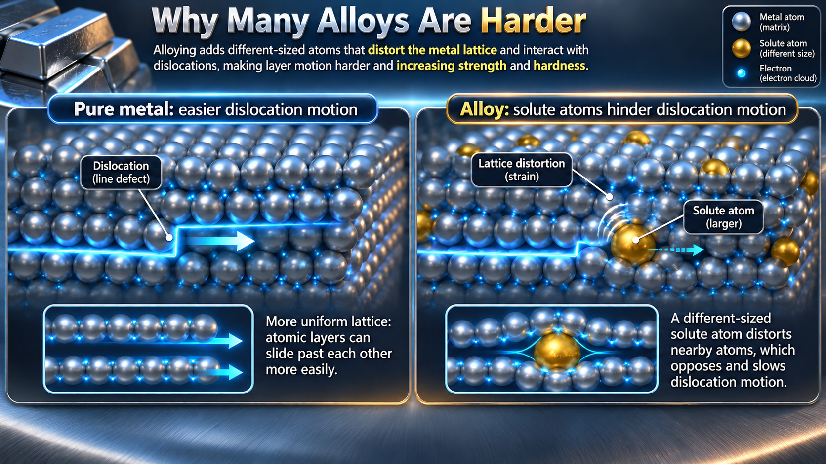
Alloys hinder dislocation motion
Qualitative lattice views show different-sized solute atoms disturbing the lattice and hindering dislocations.
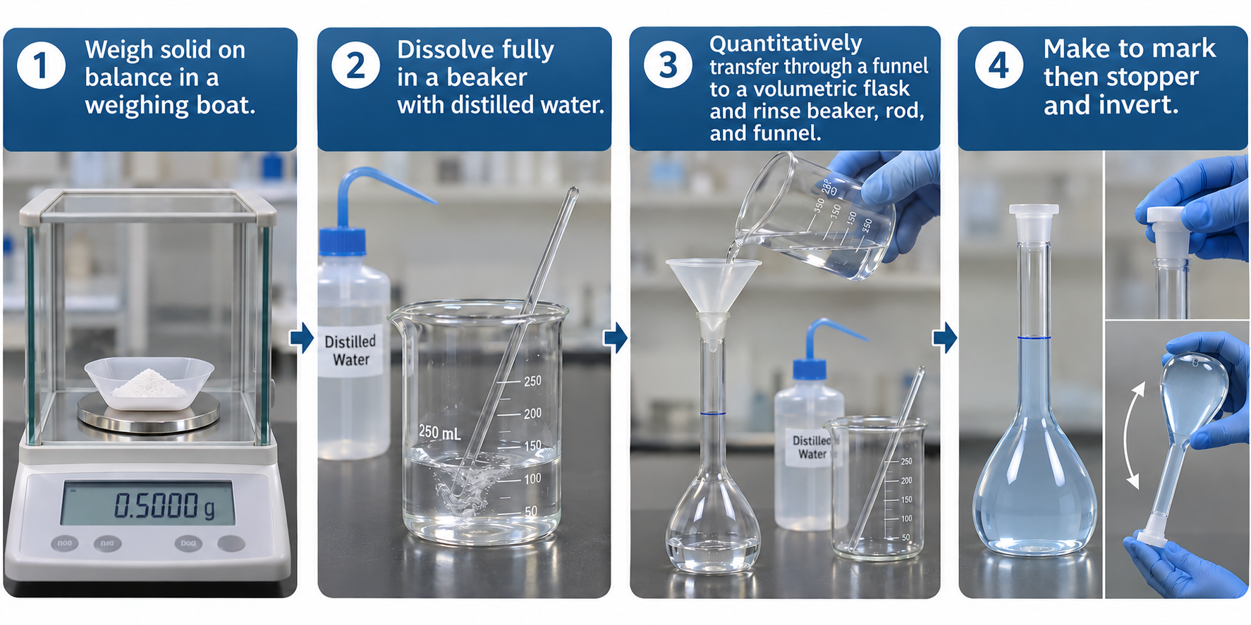
 CHEMISTRY · 5 VISUALSMaking a standard solutionA standard solution needs a known amount of solute in a known final volume. These images focus on quantitative transfer, the calibration mark and mixing.
Preparing a standard solution
Four stages show weighing, dissolving, transferring and making up to the calibration mark.
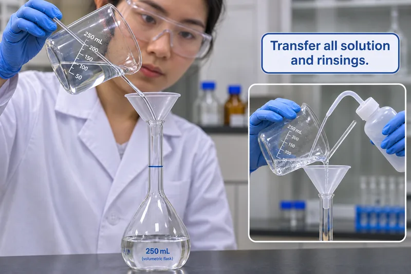
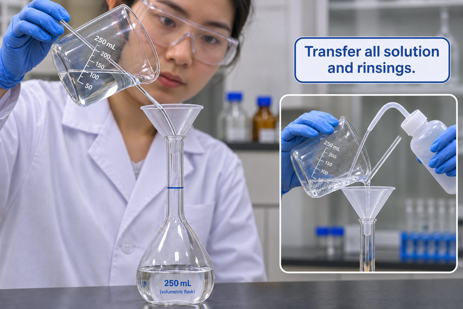
Quantitative transfer and rinsing
A beaker, glass rod and funnel guide solution into a volumetric flask; an inset shows rinsing.
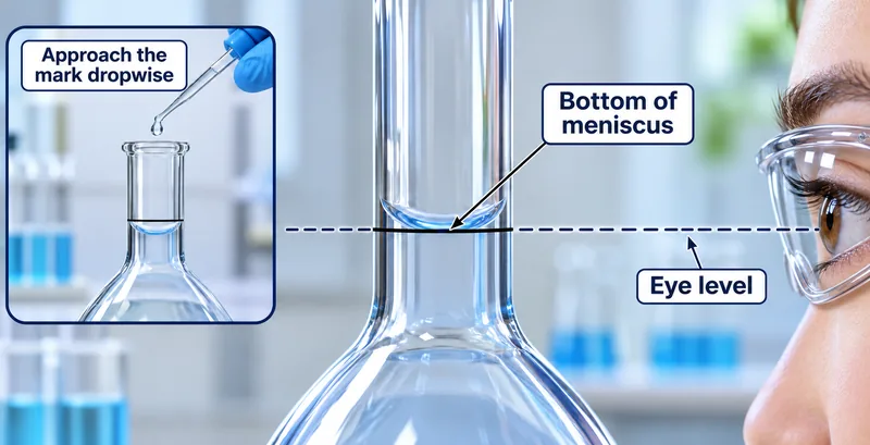
Reading the meniscus
An eye-level view aligns the bottom of a concave meniscus with the flask mark; an inset shows dropwise addition.


Sodium carbonate worked example
Preparing 250.0 mL of 0.1000 mol per litre solution requires 2.650 g of anhydrous sodium carbonate.

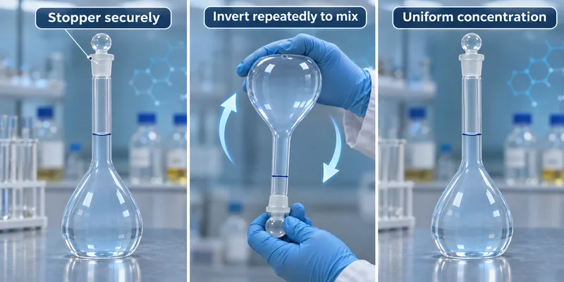
Mixing by inversion
A stoppered volumetric flask is inverted repeatedly to mix the prepared solution.

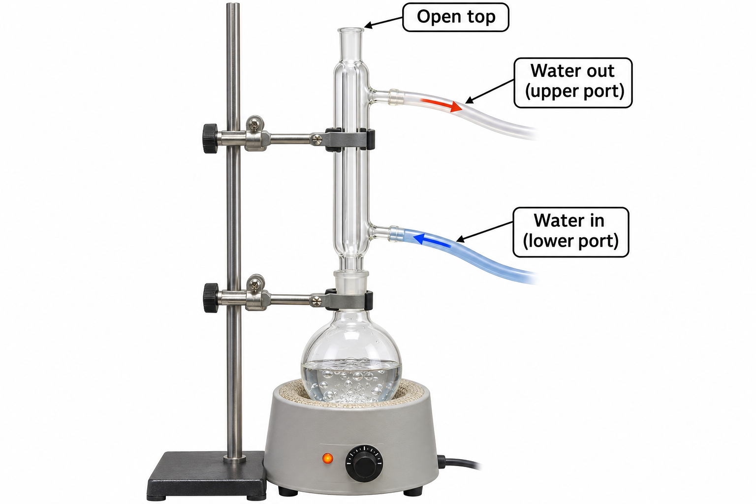
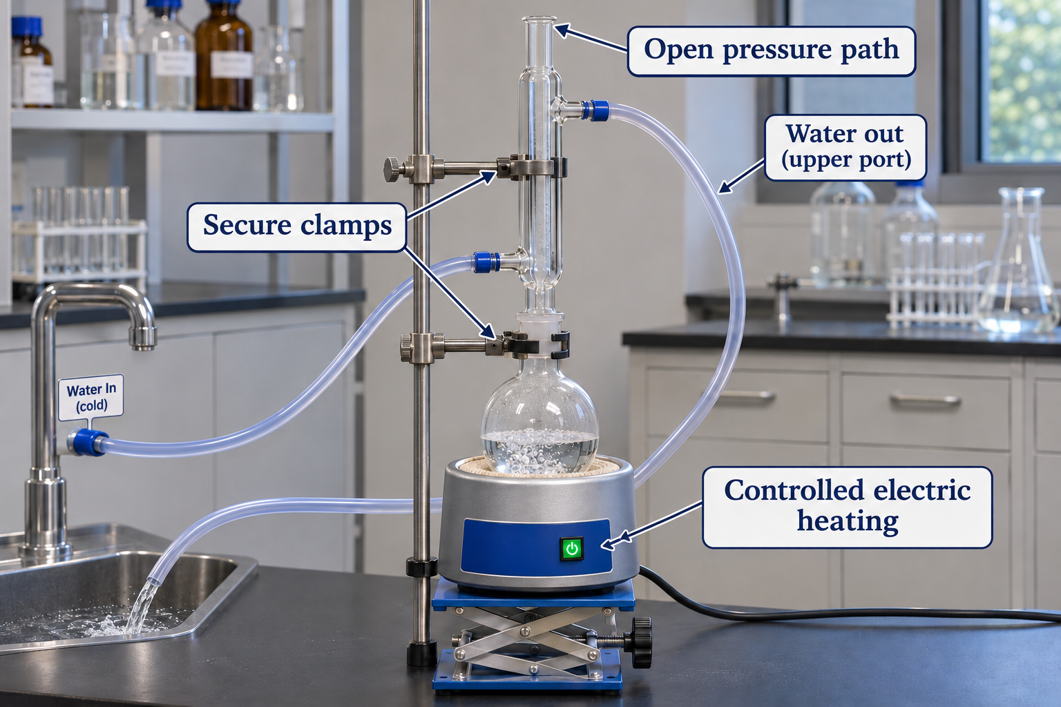
 CHEMISTRY · 5 VISUALSReflux apparatusReflux allows heating while much of the vapour condenses and returns to the reaction flask. The cooling-water jacket is separate from the reaction pathway.
A reflux apparatus overview
A vertical condenser above an electrically heated flask has lower water inlet, upper outlet and open top.
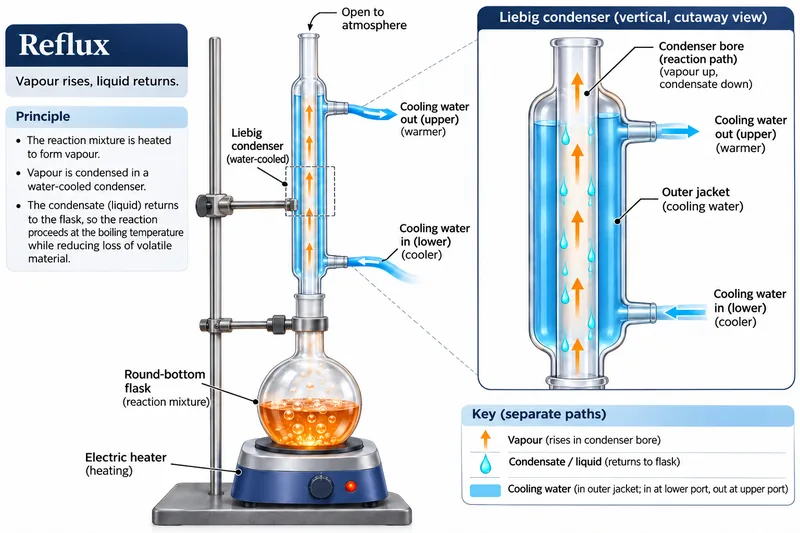
Separate paths inside a condenser
A labelled cutaway distinguishes rising vapour and returning liquid in the bore from cooling water in the jacket.


Condensation close-up
An enlarged condenser view shows rising vapour, falling condensate and the separate cooling-water jacket.


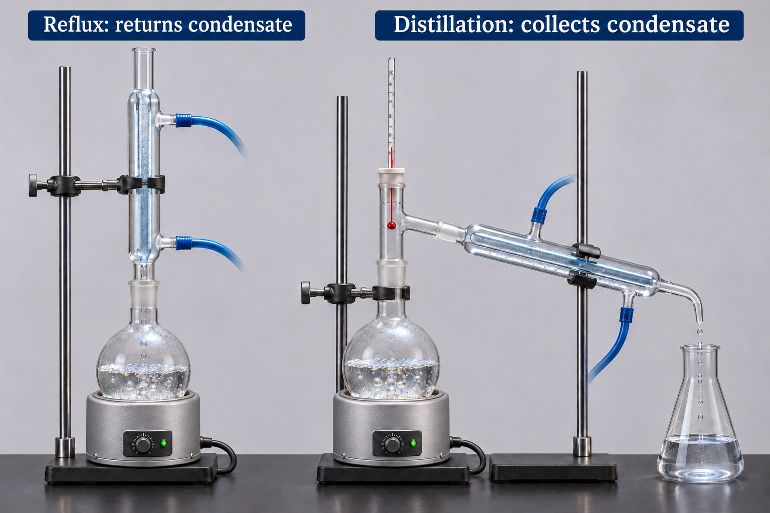
Reflux compared with distillation
Side-by-side apparatus returns condensate to a reflux flask or collects it in a distillation receiver.

Reflux connections on a bench
An electrically heated setup highlights clamps, lower cooling-water inlet, upper outlet and an open pressure path.
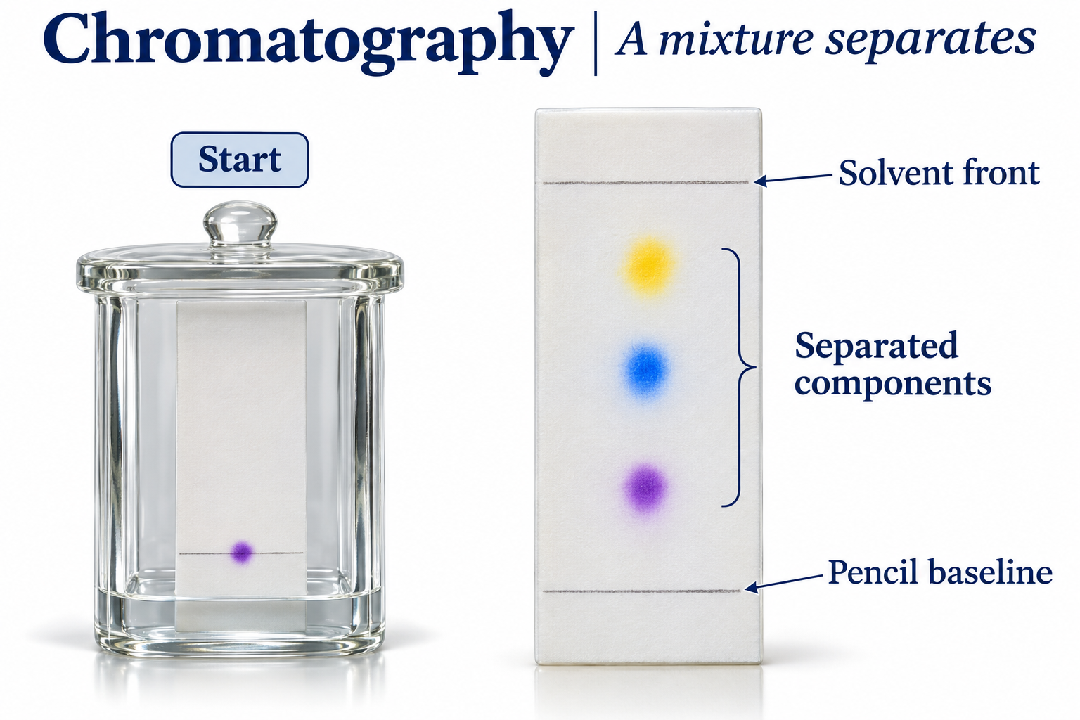
 CHEMISTRY · 5 VISUALSChromatography and RfChromatography separates mixture components by their interactions with the mobile and stationary phases. Rf compares the distance a spot moves with the solvent front.
Separating a mixture
A developing chamber and separated coloured spots identify the pencil baseline and solvent front.

Calculating Rf from one baseline
A spot moves 3.0 cm while solvent moves 6.0 cm, giving Rf = 0.50.


Mobile and stationary phases
A conceptual silica TLC view compares stronger retention at the surface with greater movement in the solvent.

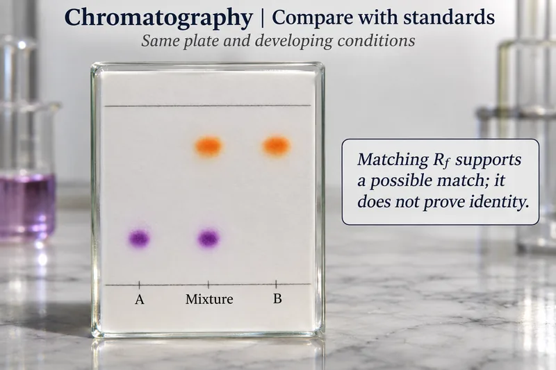
Comparing a mixture with standards
Spots from a mixture line up with standards A and B under the same developing conditions.


Two spots, two Rf values
An illustrative chromatogram gives blue Rf = 0.25 and yellow Rf = 0.75 from an 8.0 cm solvent front.

 CHEMISTRY · 5 VISUALSAtoms and ions: changing sizeForming an ion changes electron number, not proton number. These qualitative comparisons link shell occupancy, nuclear charge and ionic size.
Atoms becoming ions
Sodium loses an electron and becomes smaller; chlorine gains an electron and becomes larger in a qualitative comparison.
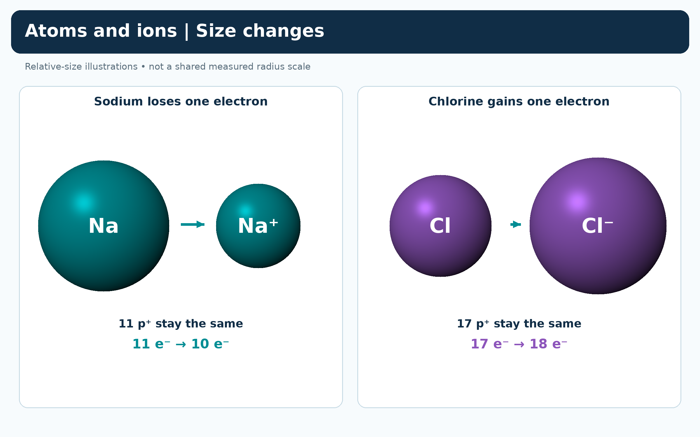

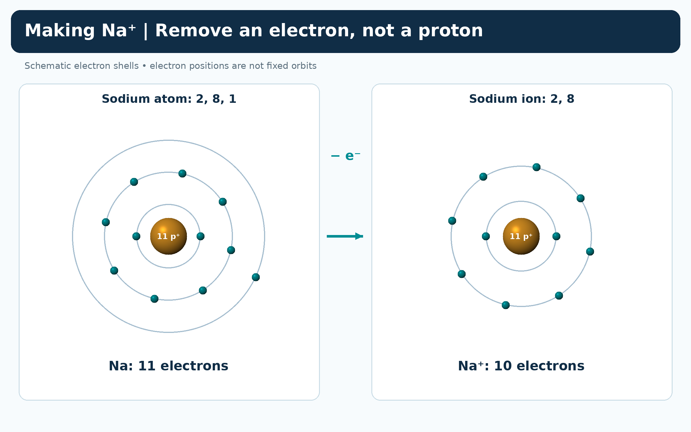
Sodium loses one electron
Shell diagrams compare sodium 2,8,1 with Na+ 2,8 while both nuclei retain eleven protons.

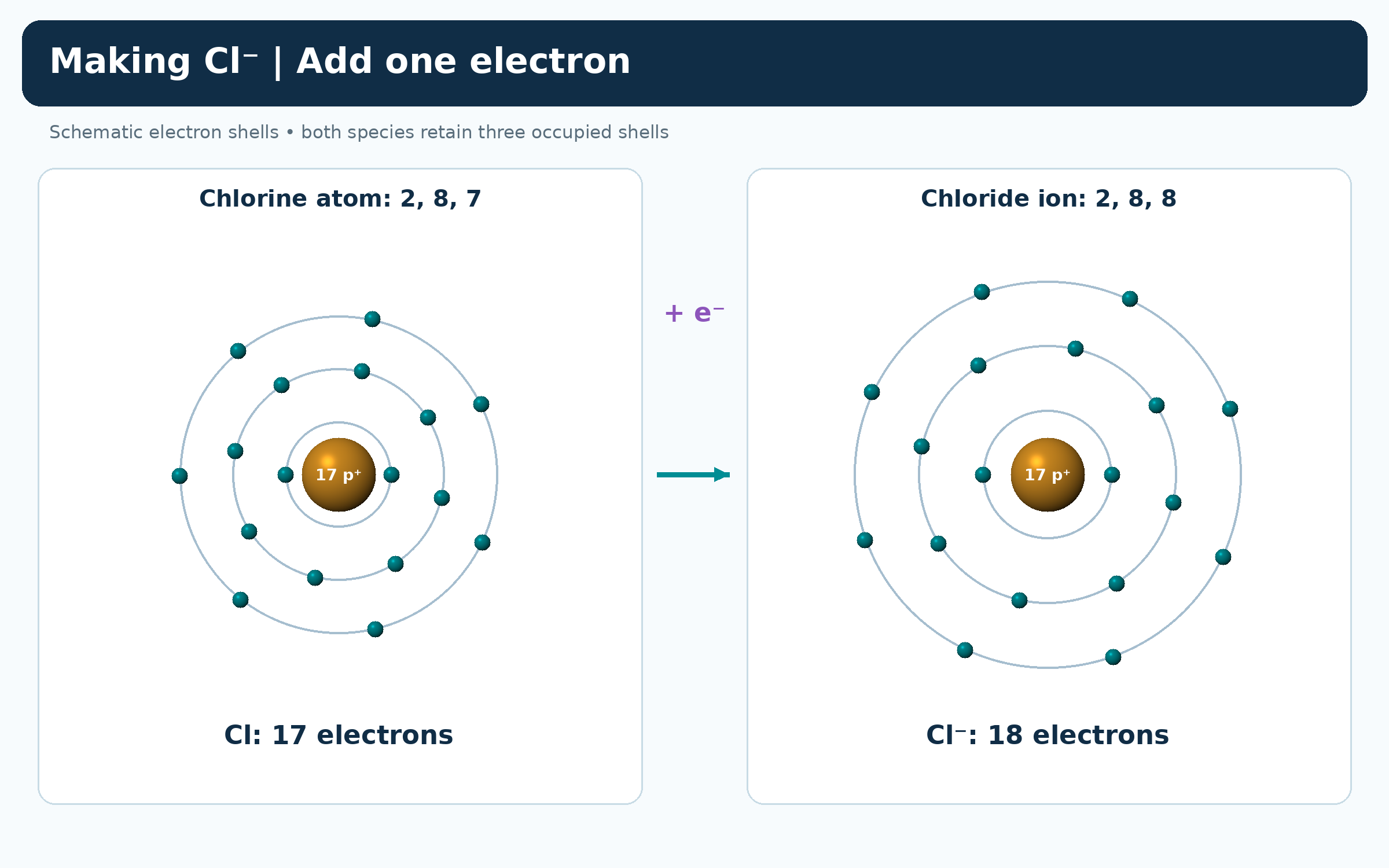
Chlorine gains one electron
Shell diagrams compare chlorine 2,8,7 with chloride 2,8,8 while both nuclei retain seventeen protons.

An isoelectronic series
O2−, F−, Na+, Mg2+ and Al3+ share ten electrons but decrease in qualitative radius as nuclear charge increases.


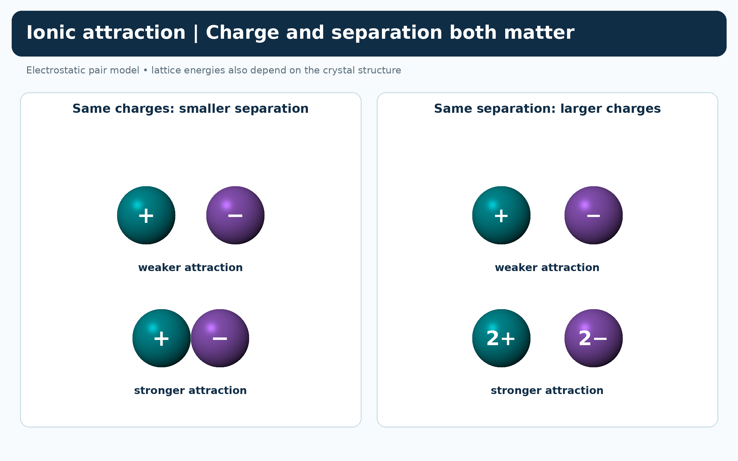
Charge and separation affect attraction
Pairs of ions compare stronger attraction at smaller separation and with larger charges.
 CHEMISTRY · 5 VISUALSElectronegativity trendsElectronegativity describes attraction for shared electrons in a bond. Periodic patterns help explain bond polarity, but bonding is not divided by a universal numerical cutoff.
Unequal sharing in HCl
Hydrogen 2.20 and chlorine 3.16 illustrate attraction towards chlorine and the resulting partial charges.

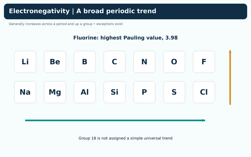
A broad periodic trend
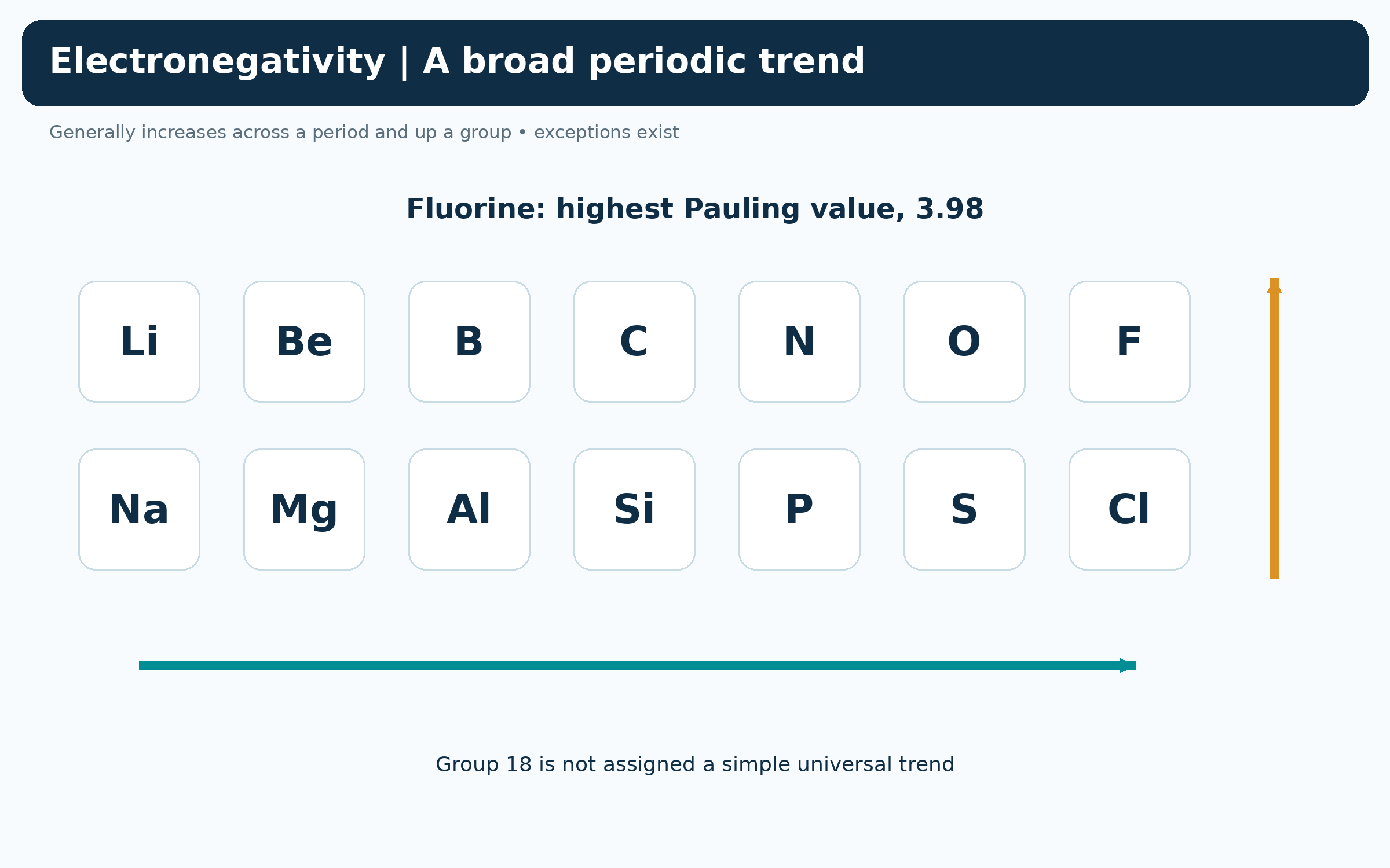
Selected period-two and period-three elements show electronegativity generally increasing across and up the table.

Comparing Pauling values
A bar chart compares hydrogen, carbon, chlorine, oxygen and fluorine on the Pauling scale.


Reading bond-dipole arrows
H–Cl and C–O bond fragments show arrows from the positive end towards the more electronegative atom.


A bonding continuum
Cl–Cl, H–Cl and ions in sodium chloride contrast equal sharing, unequal sharing and ionic bonding.

 CHEMISTRY · 5 VISUALSAtomic emission and absorptionAtoms absorb or emit photons when they change between allowed energy levels. Line spectra connect these energy gaps with characteristic wavelengths.
Absorption raises atomic energy
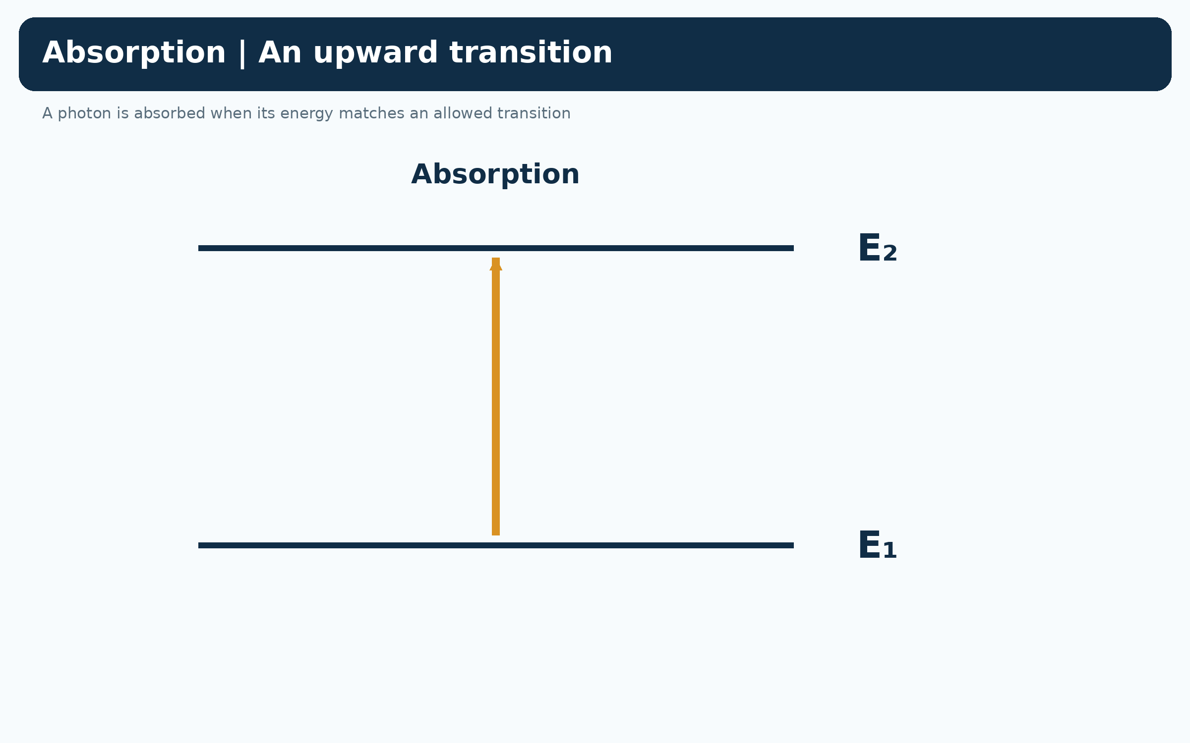
An upward arrow connects lower level E1 to higher level E2 when a matching photon is absorbed.

Emission lowers atomic energy
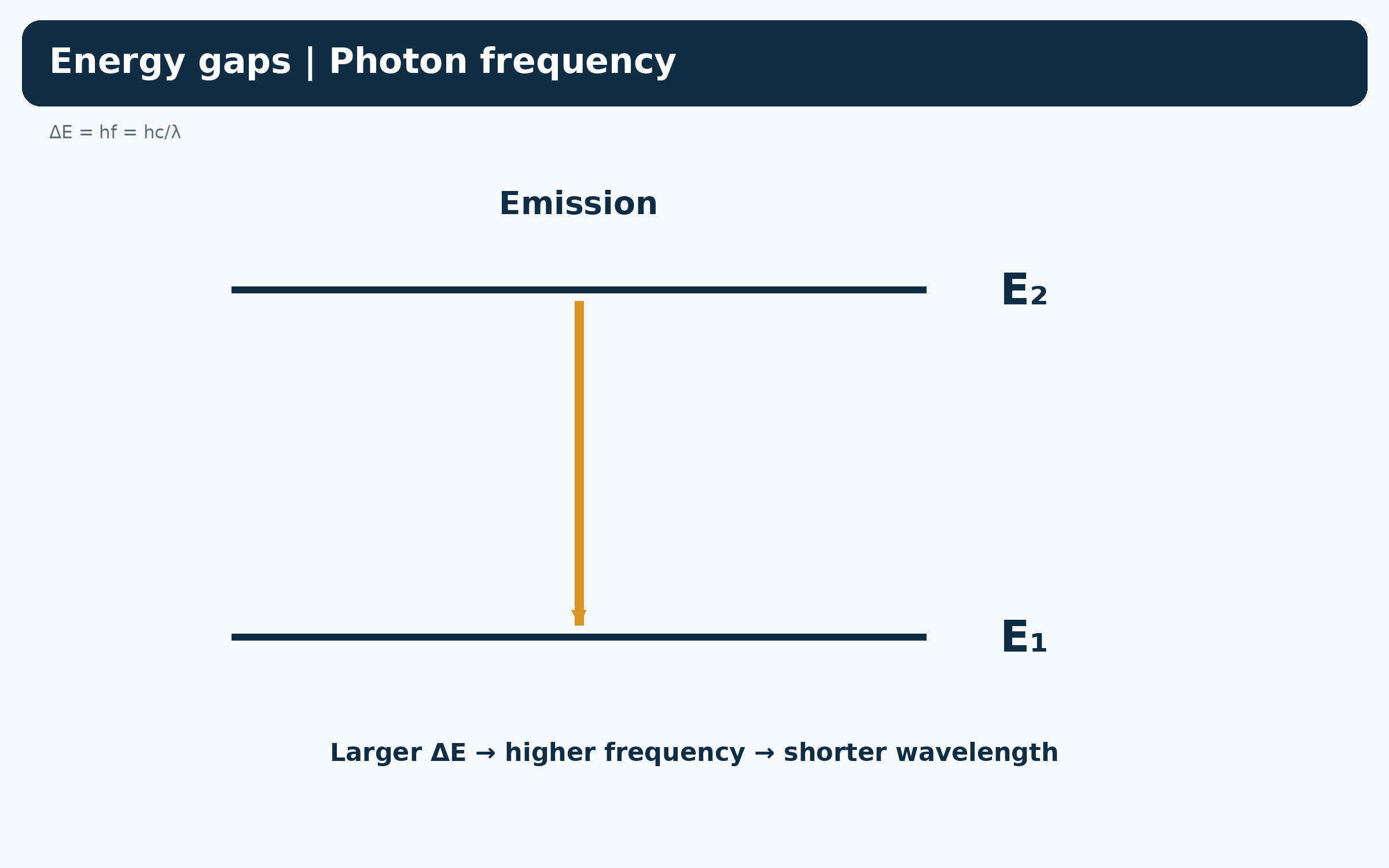
A downward arrow connects E2 to E1 as the atom emits a photon.


Energy gap and photon wavelength
An emission diagram relates energy gap to hf and hc/lambda: larger gaps mean shorter wavelengths.
Visible hydrogen Balmer lines
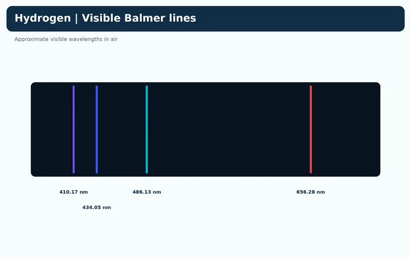
Four illustrative lines are labelled with approximate air wavelengths 410.17, 434.05, 486.13 and 656.28 nm.


Emission and absorption lines
Bright emission lines and dark absorption lines align at matching characteristic wavelengths.

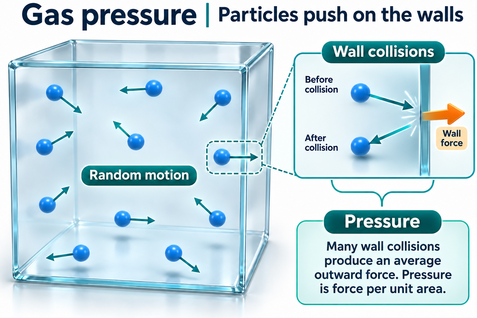
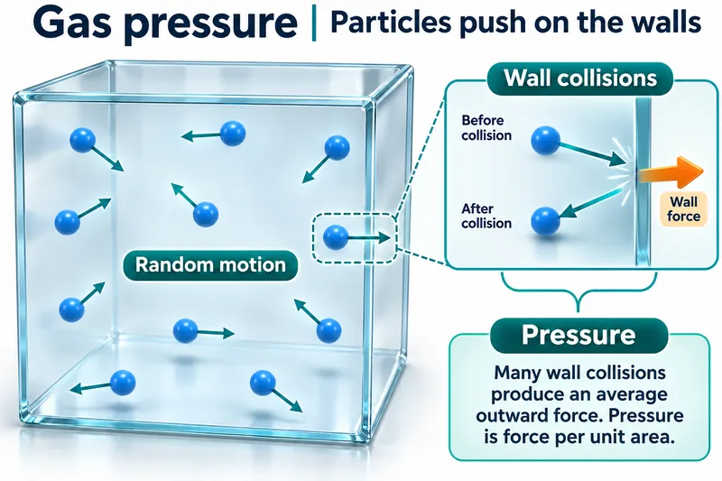 CHEMISTRY · 5 VISUALSGas pressure from particle collisionsGas pressure is the average force per unit area arising from particle collisions with walls. Ideal-gas comparisons explain changes with volume and temperature.
Particles collide with walls
Moving particles in a container and a wall-collision inset link random motion to pressure.

Momentum change at a wall
Before, during and after views show an ideal elastic collision and equal opposite forces on particle and wall.

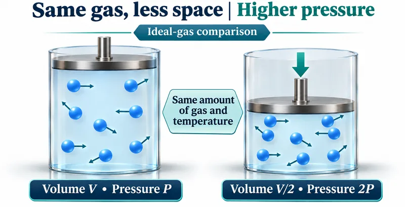
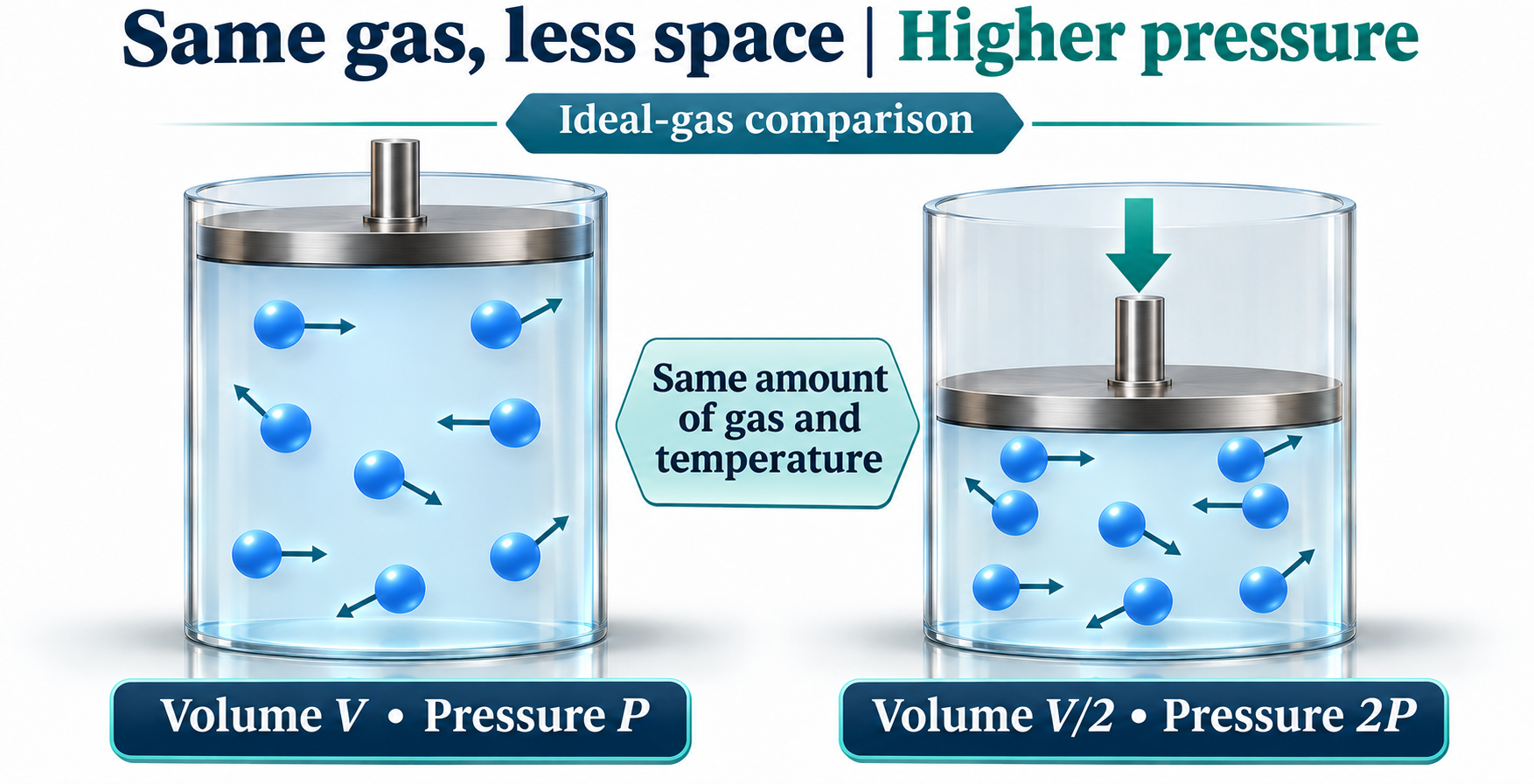
Compressing a fixed amount of gas
At the same temperature, halving volume doubles ideal-gas pressure.
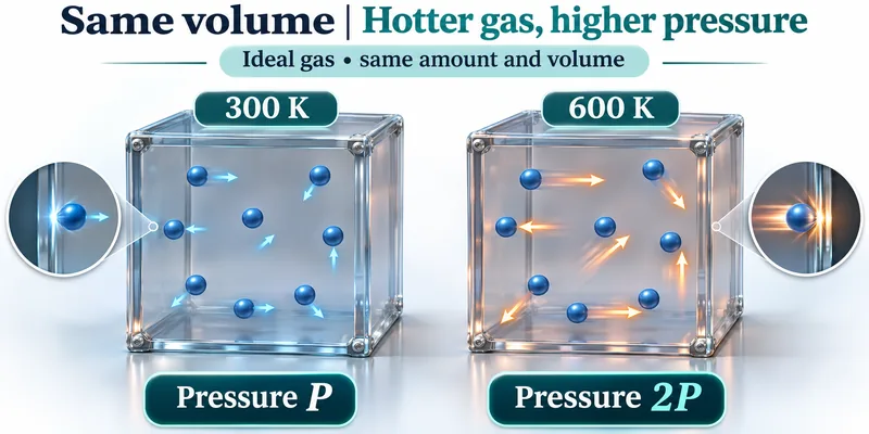
Heating gas at fixed volume
A fixed amount of ideal gas at 300 K and 600 K illustrates doubled pressure at doubled absolute temperature.
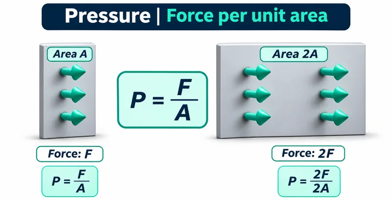
Pressure is force per unit area
Areas A and 2A receive forces F and 2F, illustrating equal pressure in both cases.
 CHEMISTRY · 5 VISUALSReaction rate factorsReaction rate depends on successful collisions, not simply the presence of reactants. The set compares concentration, temperature, surface area and catalysis.
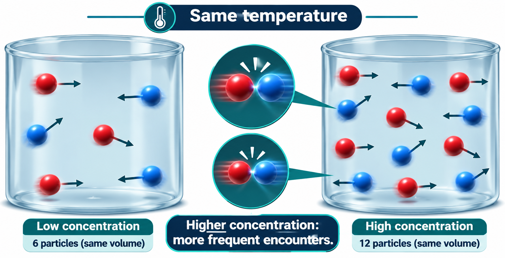
Concentration and encounters
Equal-volume containers with six and twelve particles illustrate more frequent encounters at higher concentration.

Temperature and particle energy
Particle views and schematic energy distributions show a greater fraction above the activation barrier at higher temperature.

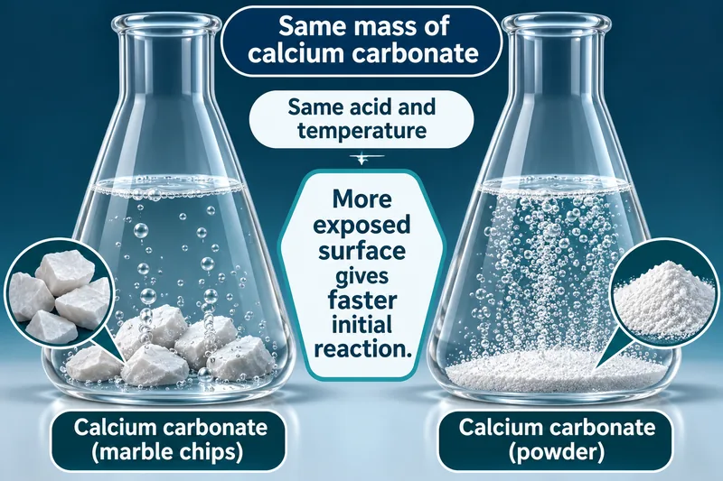
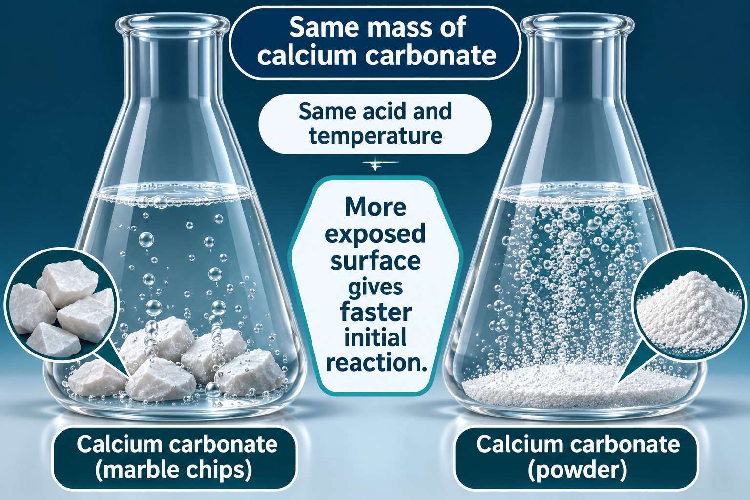
Surface area and initial rate
Equal masses of calcium carbonate chips and powder react with the same acid, with more exposed surface in the powder.
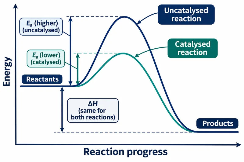
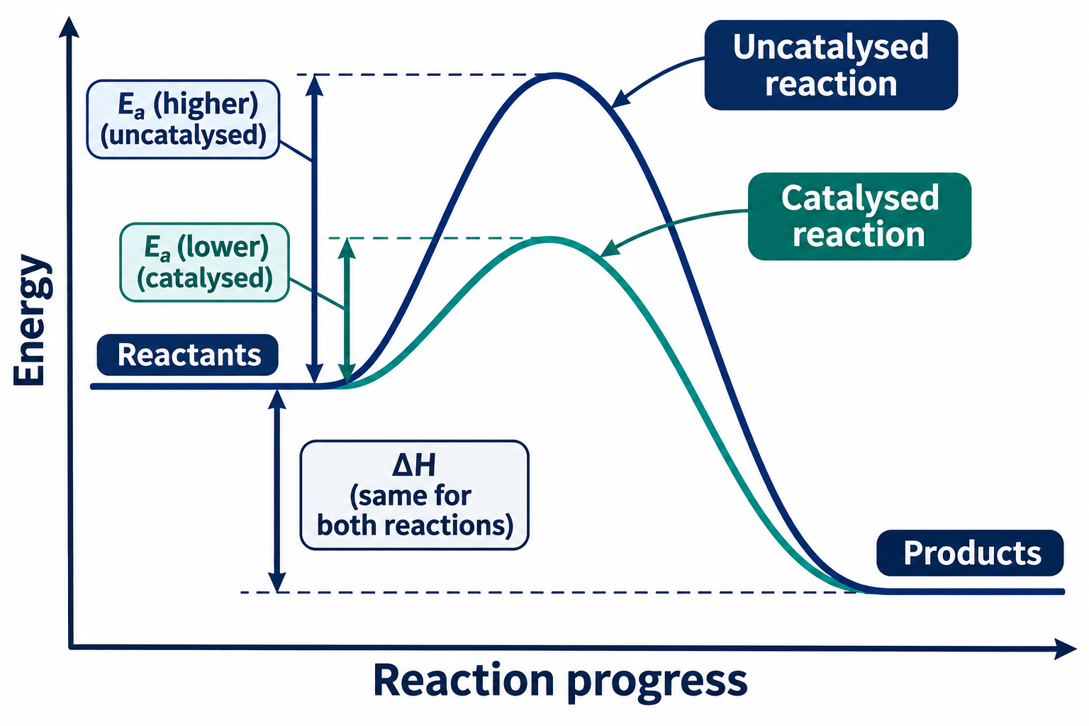
A lower activation barrier
Catalysed and uncatalysed profiles share reactant and product energies but have different activation barriers.

Successful and unsuccessful collisions
Generic A2 and B2 particles bounce apart at insufficient energy or form two AB particles in a successful collision.

 CHEMISTRY · 5 VISUALSWater phase diagramWater changes phase according to temperature and pressure. These qualitative diagrams introduce boundaries, special points and the effect of pressure on boiling.
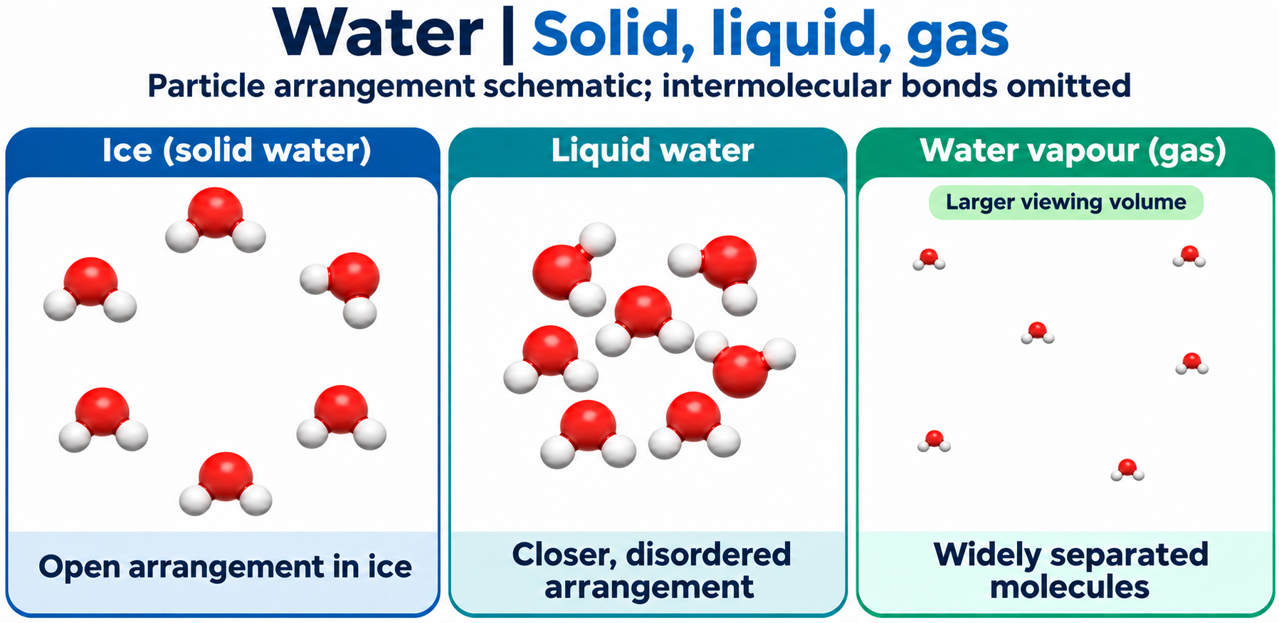
Water in three states
Schematic water molecules compare an open ice arrangement, closer disordered liquid and widely separated vapour.

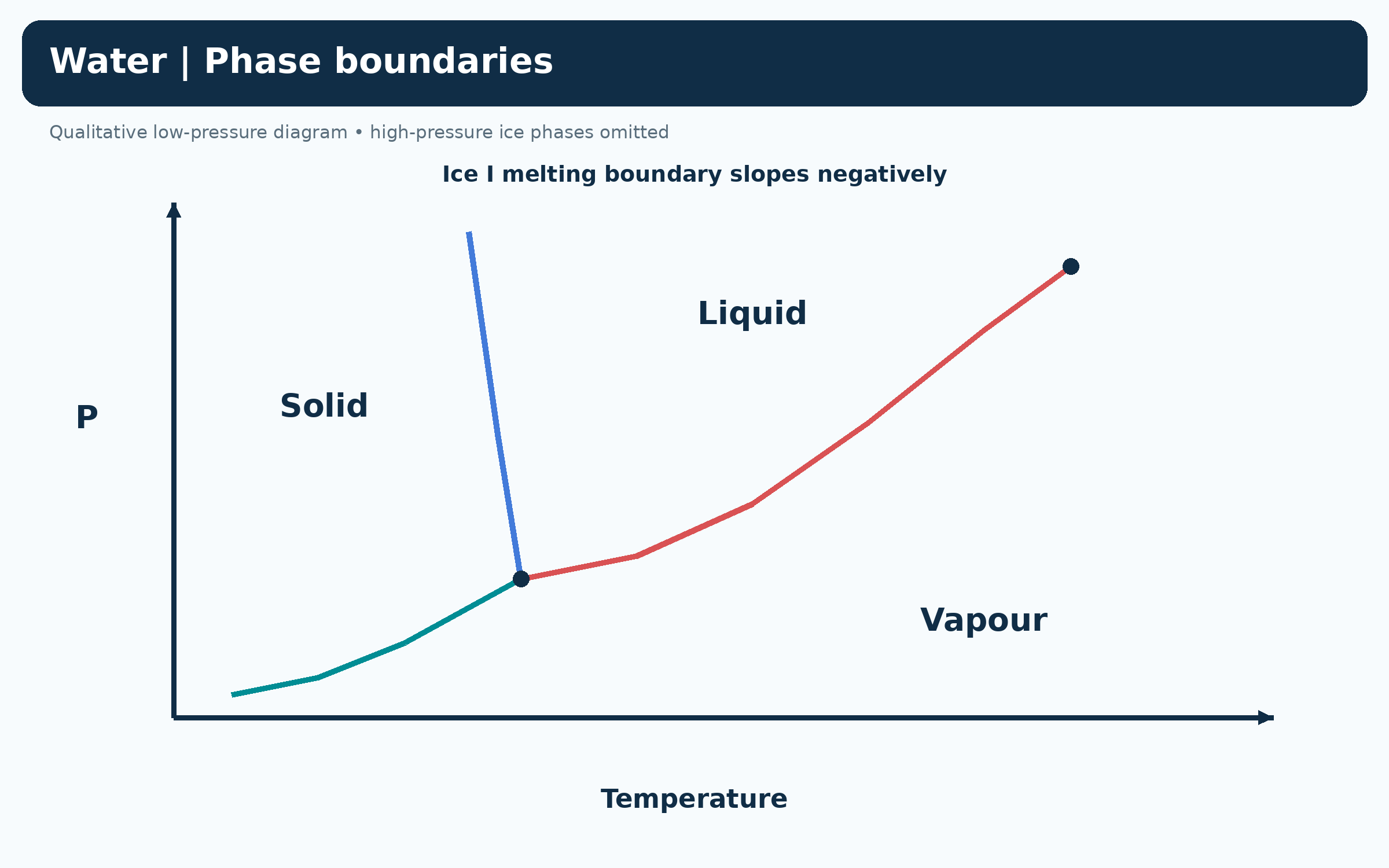
Water phase boundaries
A qualitative low-pressure diagram shows solid, liquid and vapour, with a negatively sloping ice-I melting boundary.
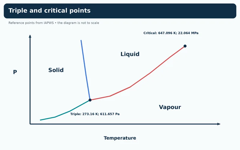
Triple and critical points
A qualitative phase diagram labels water reference triple and critical temperatures and pressures.


Heating at different pressures
Two paths contrast melting then boiling above the triple point with sublimation below its pressure.

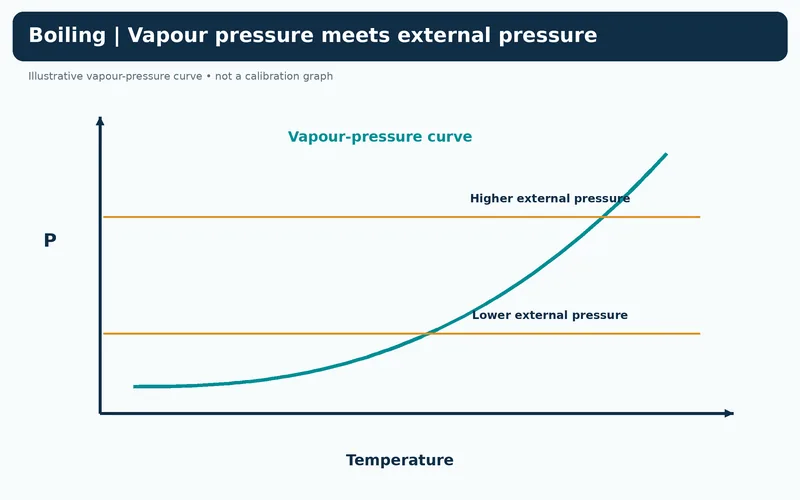
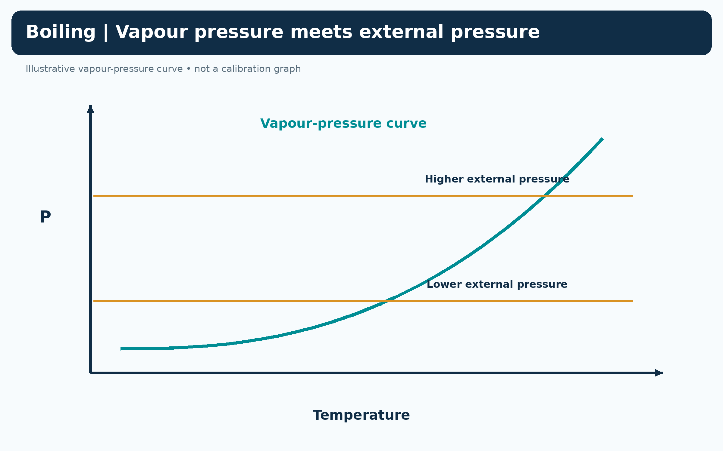
Boiling and external pressure
A qualitative vapour-pressure curve meets two external pressures at different boiling temperatures.
 CHEMISTRY · 5 VISUALSCalorimetry and heat transferCalorimetry uses temperature change to estimate energy transferred. The sign of heat for a reaction is opposite to that for its surroundings under the stated ideal assumptions.
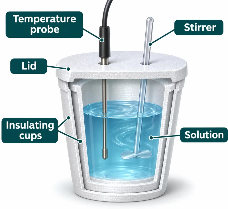
An insulated-cup calorimeter
A cutaway labels the temperature probe, stirrer, lid, insulating cups and solution.


An exothermic reaction warms solution
An insulated-cup illustration shows energy moving from the reaction to the surrounding solution.

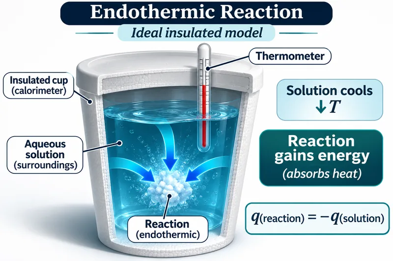
An endothermic reaction cools solution
An insulated-cup illustration shows the reaction absorbing heat from the solution.

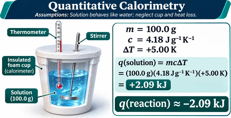
Calculating heat from temperature change
An illustrative 100.0 g solution warms by 5.00 K, giving +2.09 kJ for solution and approximately −2.09 kJ for reaction.

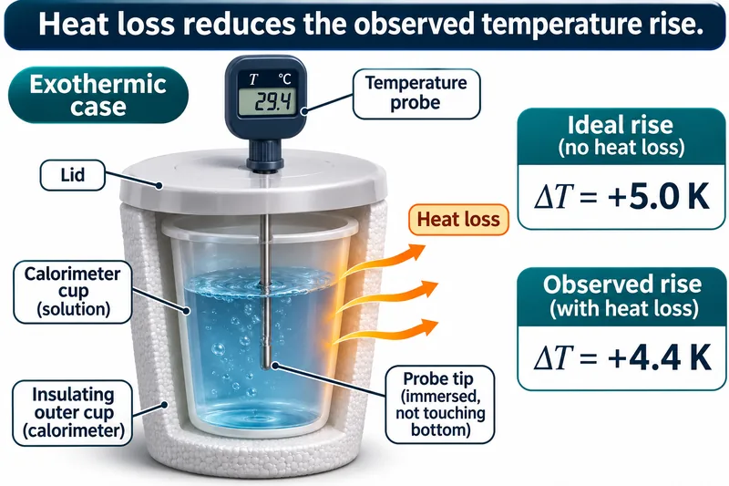
Heat loss changes the observed rise
An exothermic example contrasts an ideal 5.0 K rise with an illustrative 4.4 K rise when heat escapes.

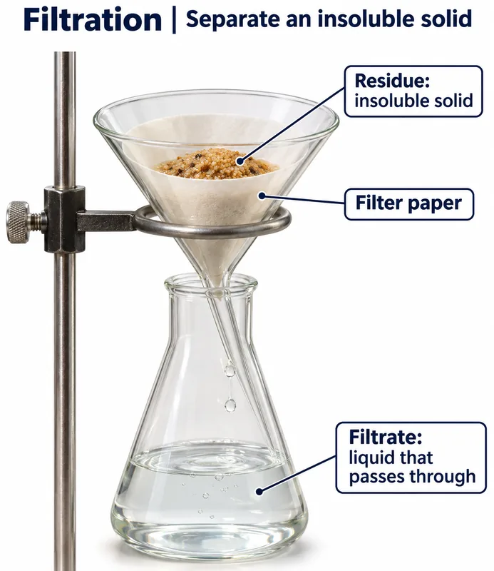 CHEMISTRY · 5 VISUALSFiltration apparatusFiltration separates an insoluble solid from a liquid. Ordinary filter paper retains sand but does not remove dissolved sodium and chloride ions.
Residue and filtrate
A funnel with filter paper retains insoluble solid while liquid collects in a flask.
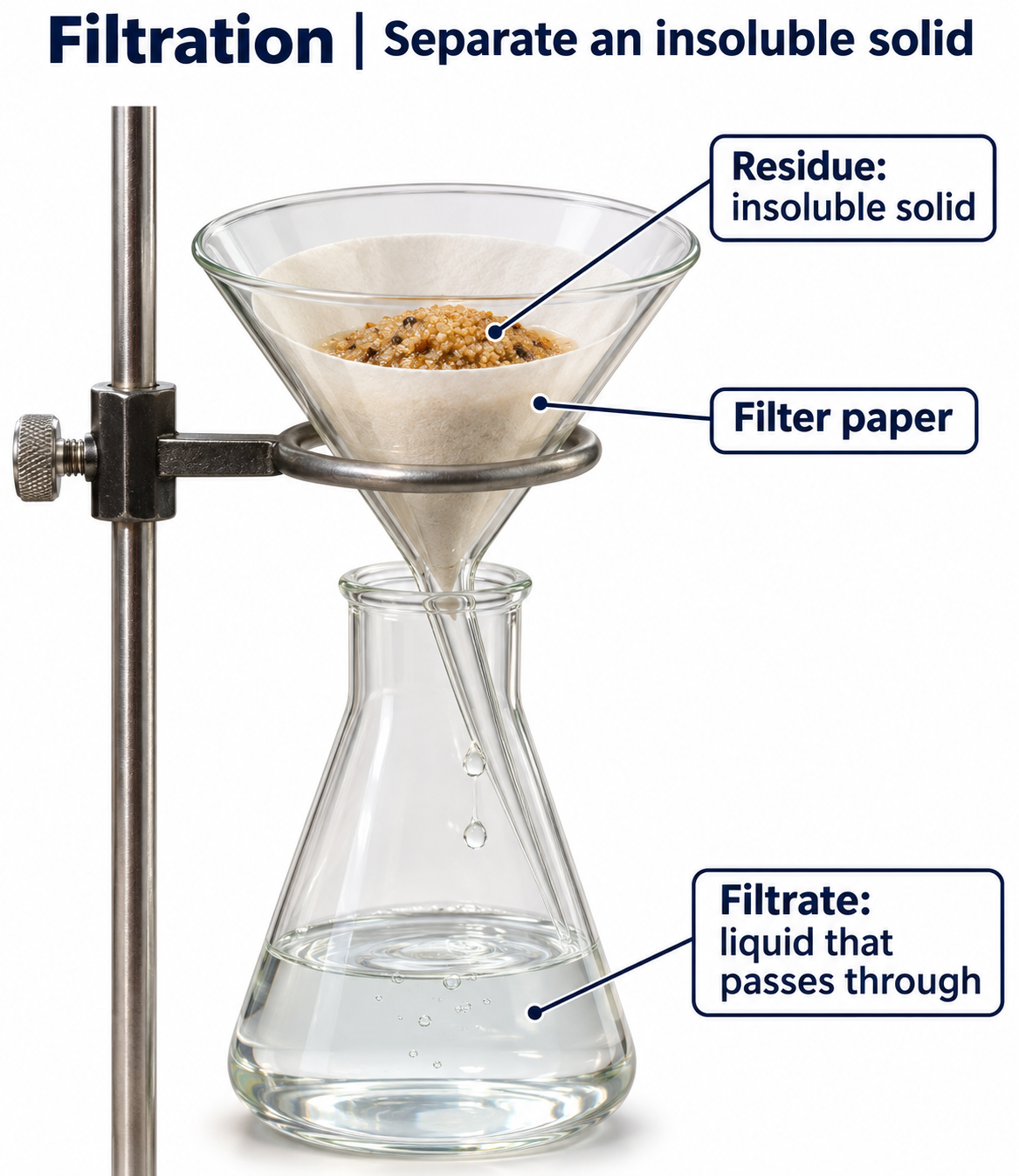
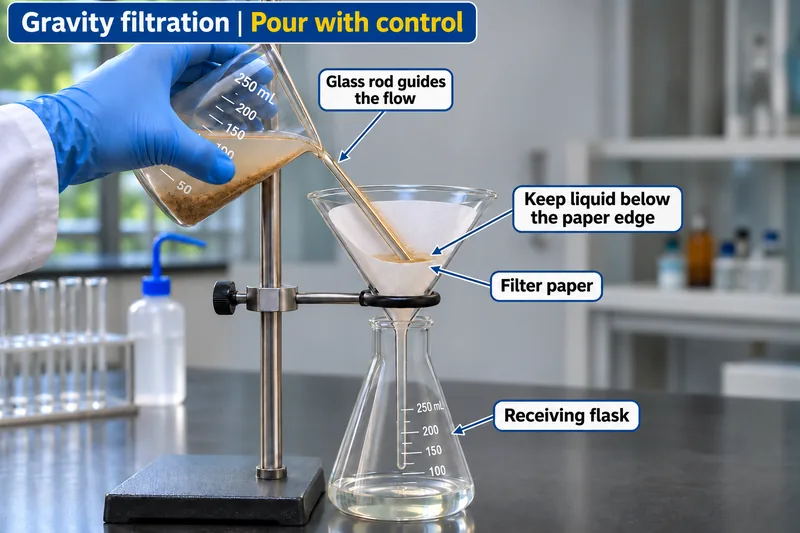
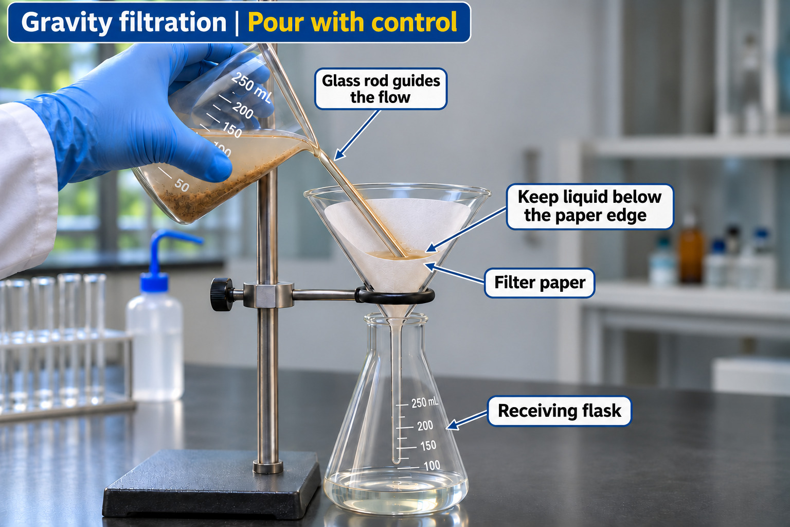
Controlled gravity filtration
A glass rod guides liquid into a paper-lined funnel while the level stays below the paper edge.

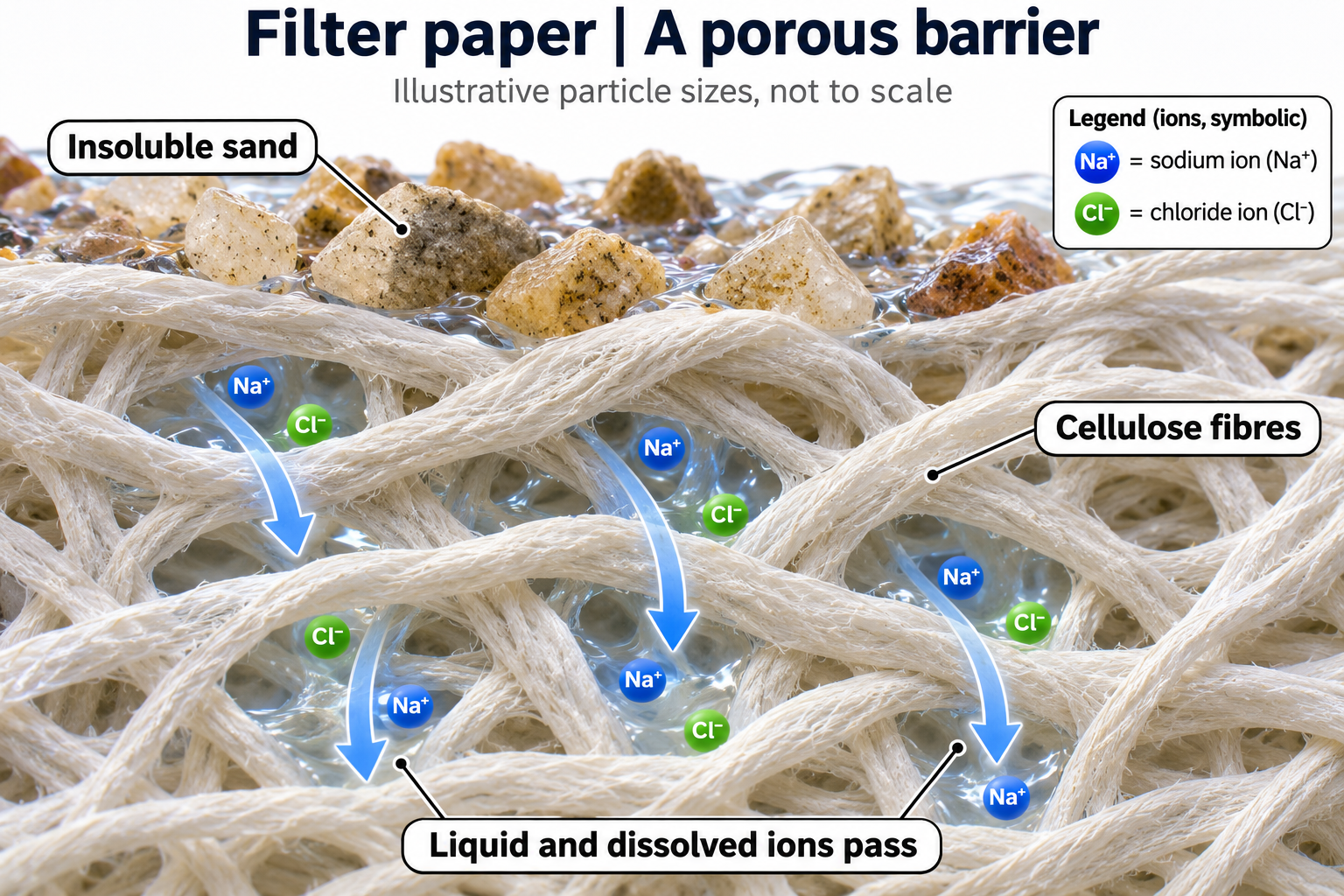
Sand stays, dissolved ions pass
An apparatus view and conceptual inset show sand retained while sodium and chloride ions pass in solution.


Gravity and vacuum filtration
Side-by-side setups compare a paper-lined glass funnel with a Buchner funnel, vacuum-rated flask and trap.


Filter paper as a porous barrier
A conceptual fibre view shows sand retained while liquid and dissolved ions pass through gaps.
 CHEMISTRY · 5 VISUALSFractional distillation apparatusFractional distillation improves separation through repeated vaporisation and condensation. The column enriches rising vapour in the more volatile component.
Fractional distillation apparatus
A boiling flask, fractionating column, condenser and receiver are shown with cooling-water direction.


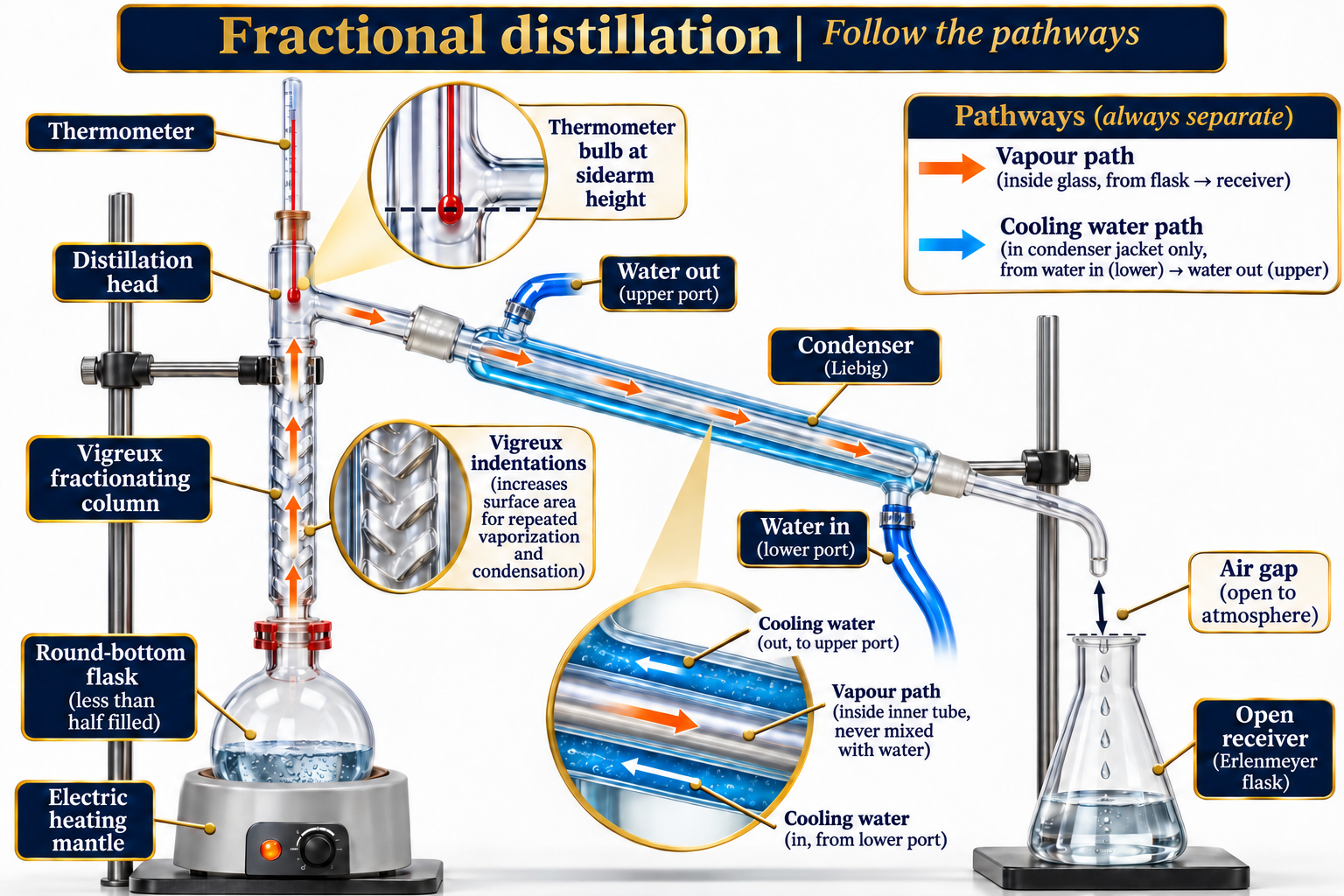
Following separate pathways
Detailed callouts distinguish vapour, distillate and cooling water, with the thermometer at sidearm height.
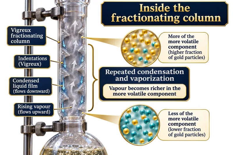
Inside a fractionating column
A Vigreux column shows rising vapour and falling liquid, with qualitative enrichment in the more volatile component.
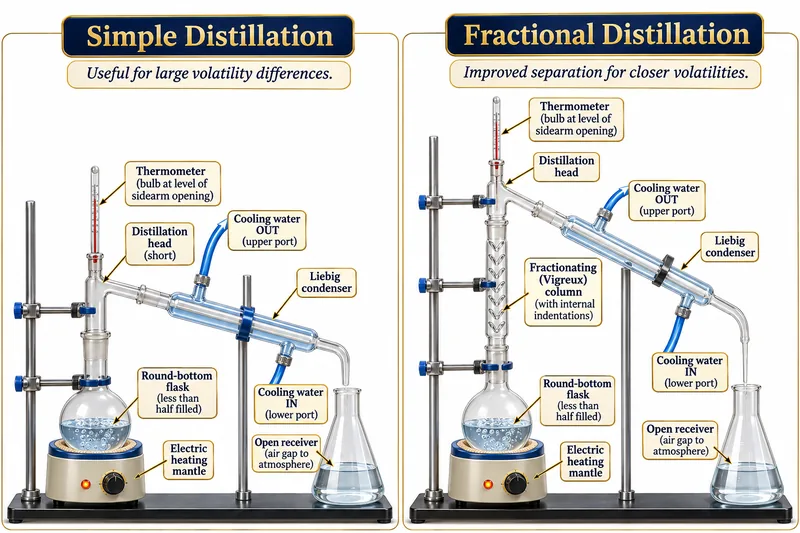
Simple and fractional distillation
Two apparatus arrangements compare separation without and with a fractionating column.
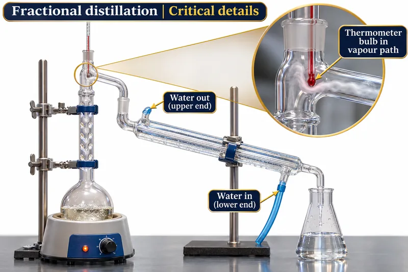
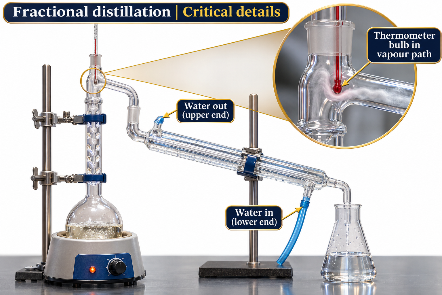
Key apparatus details
Close-ups highlight the thermometer bulb in the vapour path and lower-inlet, upper-outlet condenser water.
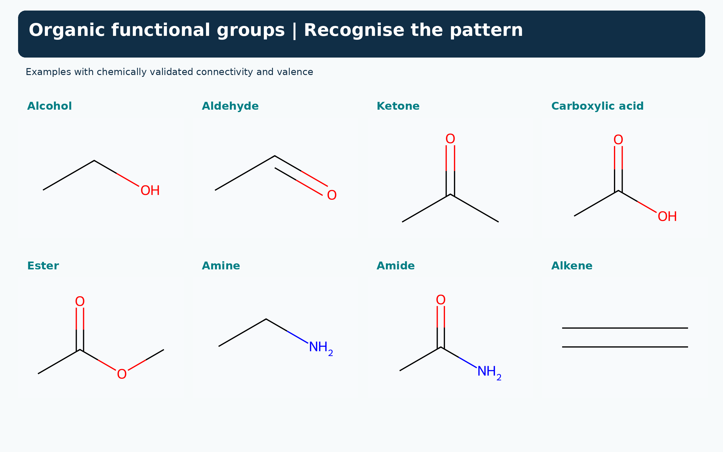
 CHEMISTRY · 5 VISUALSOrganic functional groupsFunctional groups help us recognise recurring structures and reaction patterns. The atoms beside a carbonyl distinguish several families that can otherwise look similar.
Recognising eight functional groups
Structures show alcohol, aldehyde, ketone, carboxylic acid, ester, amine, amide and alkene examples.
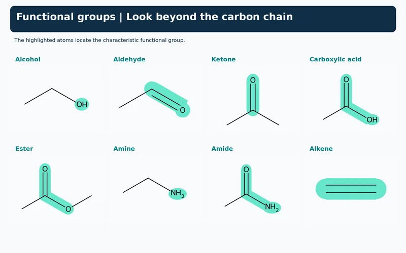
Highlighting the defining atoms
The same eight examples highlight the atoms or bond that define each functional group.


Amine compared with amide
Displayed methylamine and ethanamide compare a nitrogen without and with an adjacent carbonyl carbon.


Carbonyl groups with different neighbours
Displayed aldehyde, ketone, carboxylic acid, ester and amide examples show the groups attached to C=O.


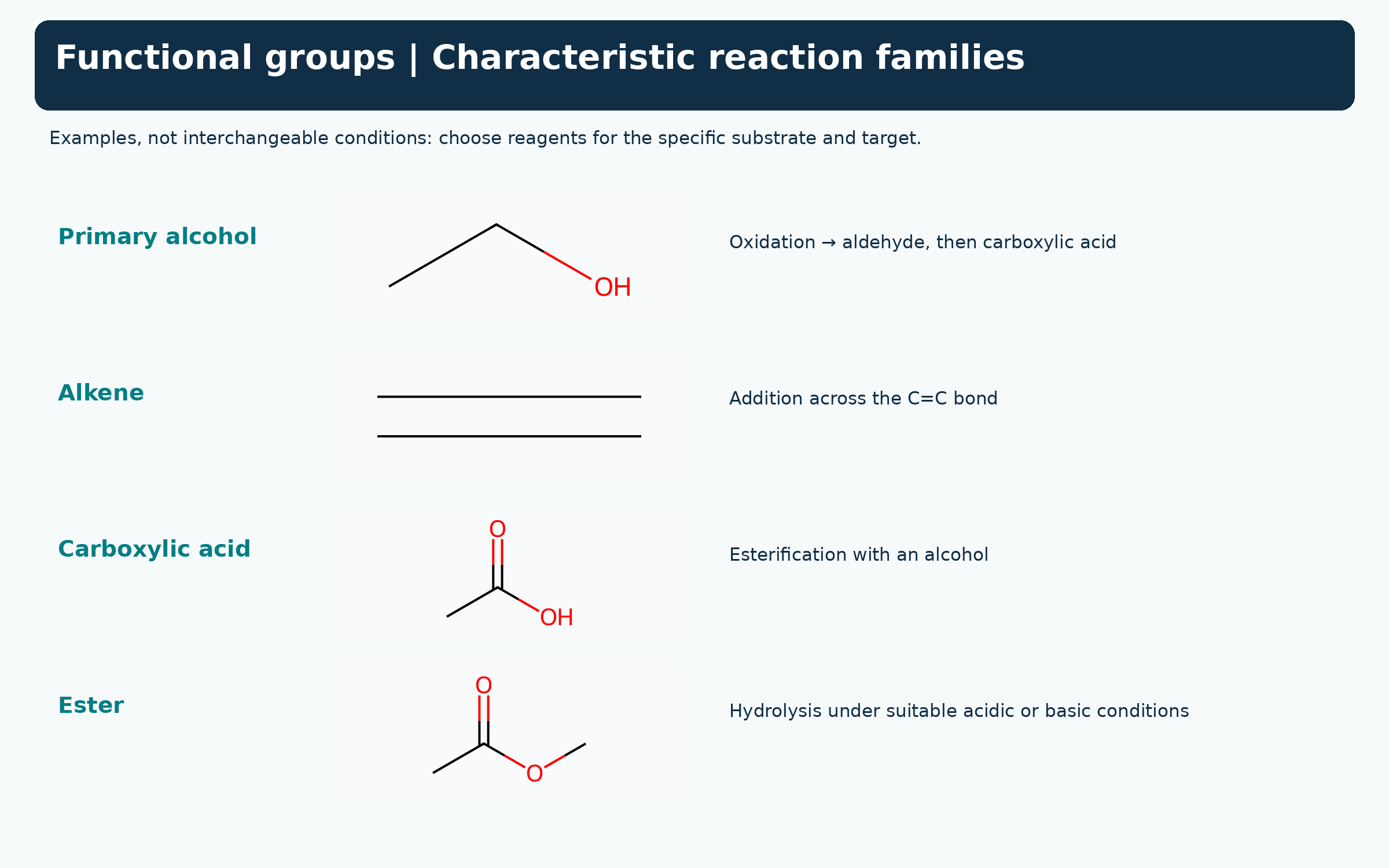
Functional groups and reaction families
Selected alcohol, alkene, carboxylic acid and ester examples link to characteristic reaction types.
 CHEMISTRY · 5 VISUALSDisplayed, condensed and skeletal formulaeDisplayed, condensed and skeletal formulae can describe the same connectivity. Reading skeletal notation means restoring implied carbon atoms and their hydrogens.
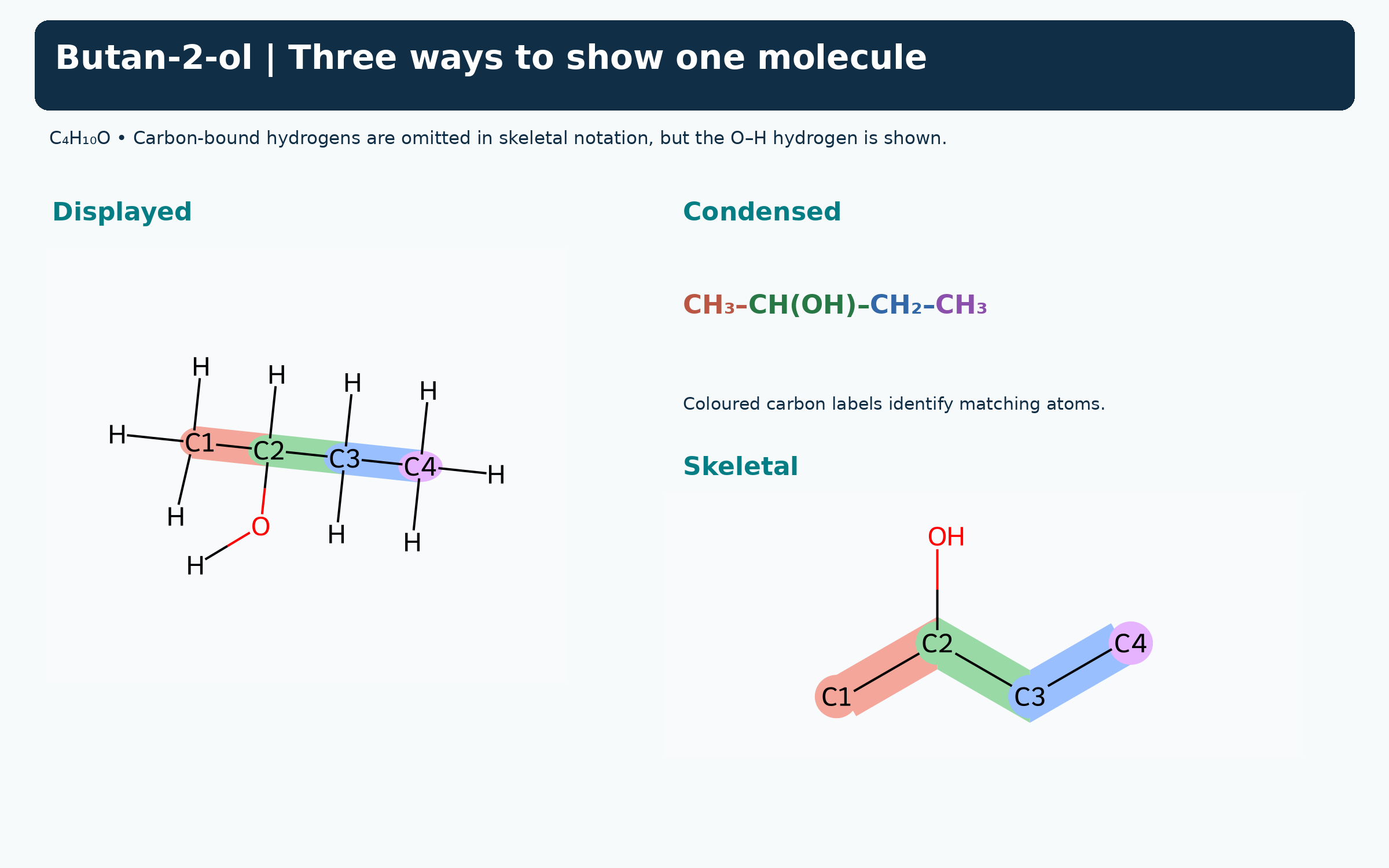
Three views of butan-2-ol
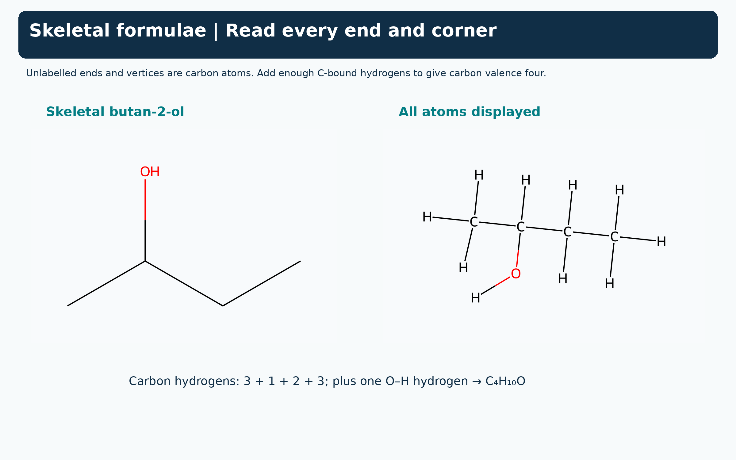
Displayed, condensed and skeletal formulae represent the same C4H10O molecule.

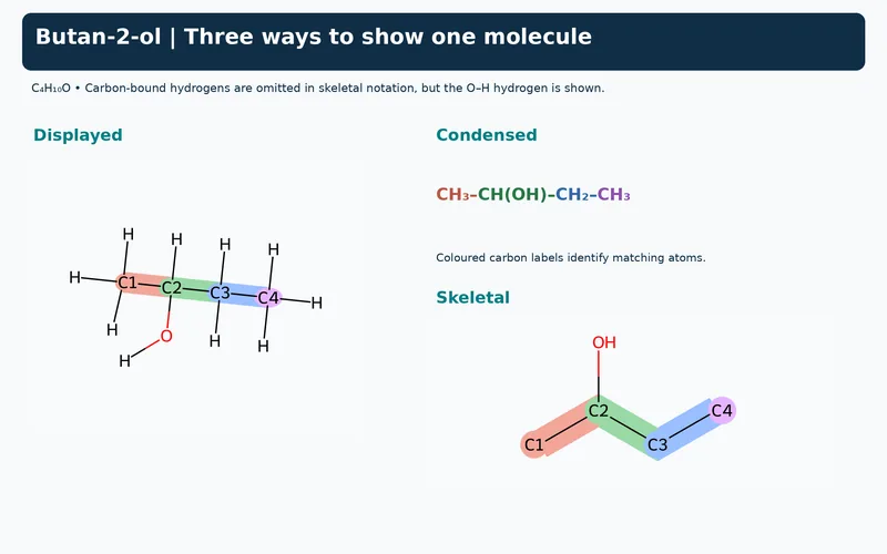
Matching carbon atoms between formulae
Colour-coded carbons connect the three representations of butan-2-ol.
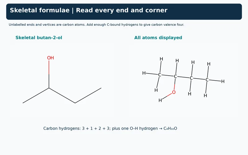
Reading skeletal ends and corners
Skeletal and fully displayed butan-2-ol illustrate implied carbons and the hydrogen count.
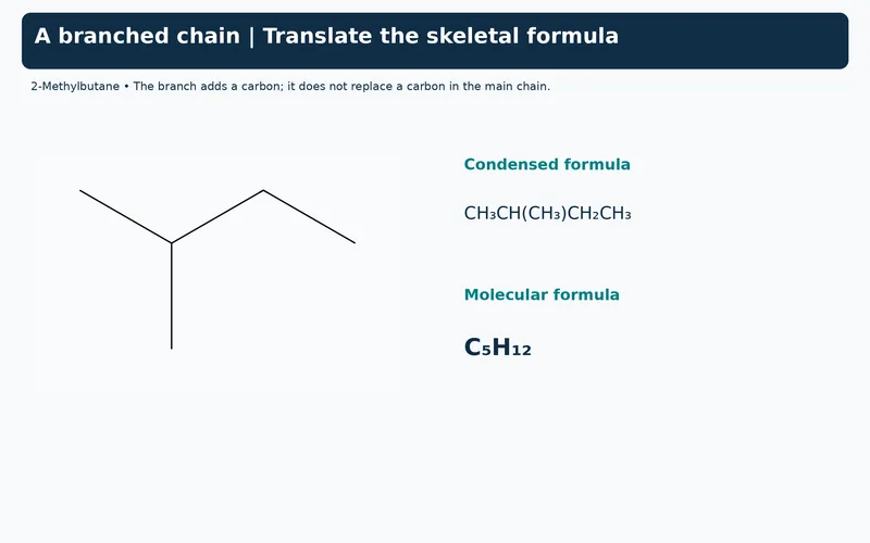
A branched chain example
Skeletal 2-methylbutane is paired with its condensed formula and molecular formula C5H12.
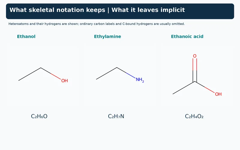
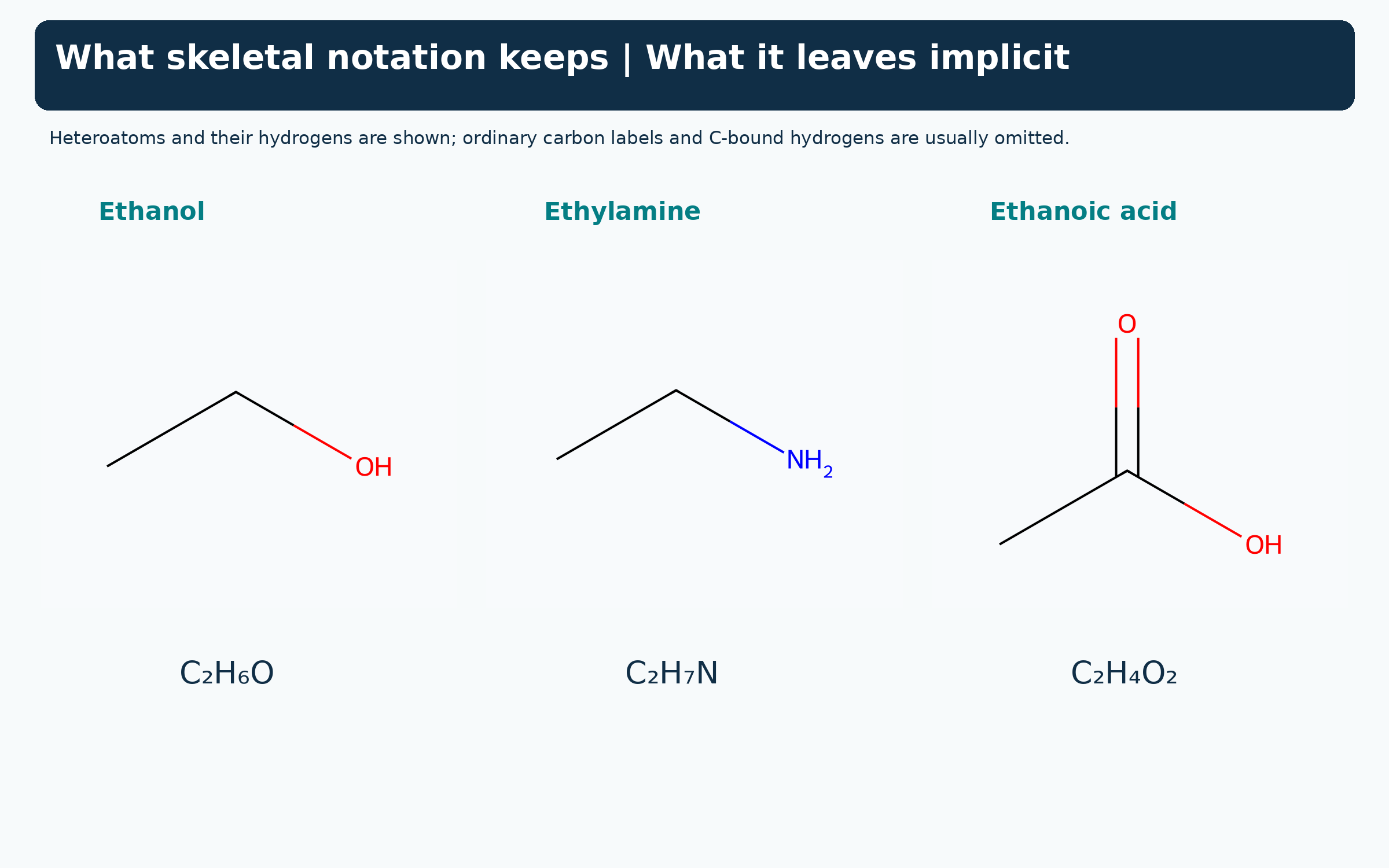
What skeletal notation retains
Ethanol, ethylamine and ethanoic acid show labelled heteroatoms and their attached hydrogens.
 CHEMISTRY · 5 VISUALSStructural and geometric isomerismIsomers share a molecular formula but differ in connectivity or spatial arrangement. These examples separate constitutional isomerism from restricted rotation at a double bond.
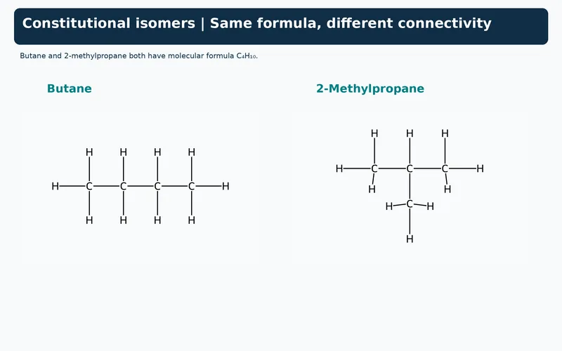
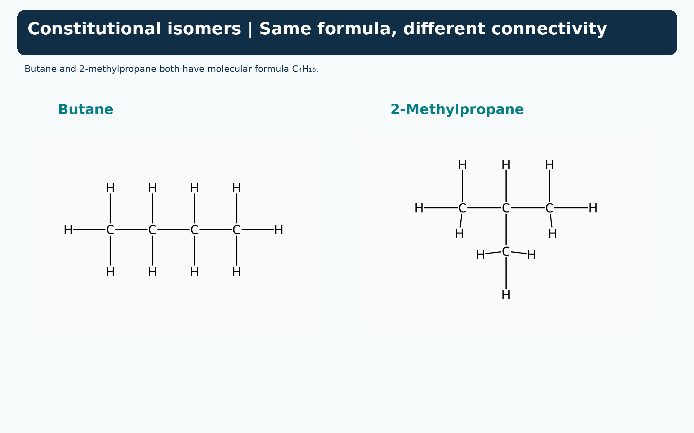
Same formula, different connectivity
Displayed butane and 2-methylpropane are constitutional isomers with formula C4H10.

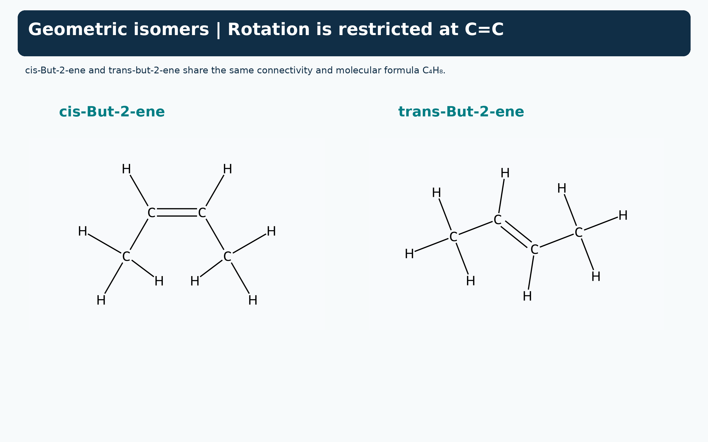
Cis and trans but-2-ene
Displayed structures compare the methyl-group positions around a restricted C=C bond.

Assigning E and Z priorities
Halogen-substituted alkenes compare higher-priority I and Br groups on the same or opposite sides.


Two kinds of isomerism
Skeletal examples contrast changed connectivity with changed arrangement around a double bond.


Three-dimensional C4H10 models
MMFF-optimised space-filling models compare anti butane with branched 2-methylpropane.

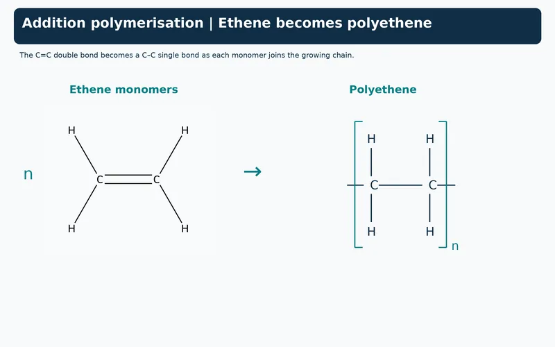 CHEMISTRY · 5 VISUALSAddition polymerizationAddition polymerisation joins alkene monomers into chains. A repeat unit describes part of that chain, so its backbone bonds continue through the brackets.
Ethene becomes polyethene
An ethene monomer equation produces a bracketed two-carbon polyethene repeat unit.


Reading repeat-unit brackets
The polyethene backbone extends through the brackets; each carbon retains four bonds.


Monomer, repeat unit and chain
Three representations distinguish ethene, a polyethene repeat unit and a short continuing chain segment.


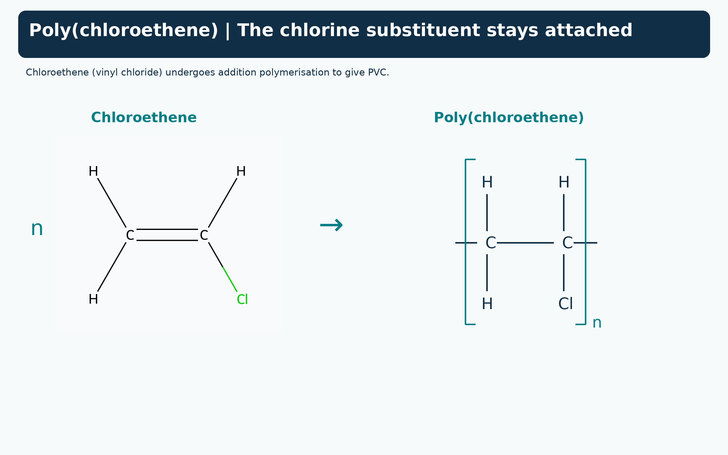
Chloroethene becomes PVC
The chlorine substituent remains attached when chloroethene forms poly(chloroethene).
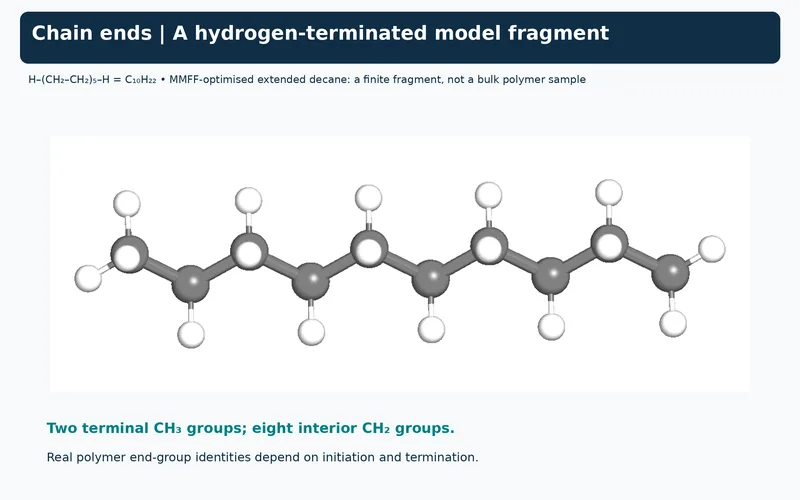
A finite hydrogen-terminated fragment
An MMFF-optimised extended decane model illustrates H–(CH2CH2)5–H, not a bulk polymer sample.

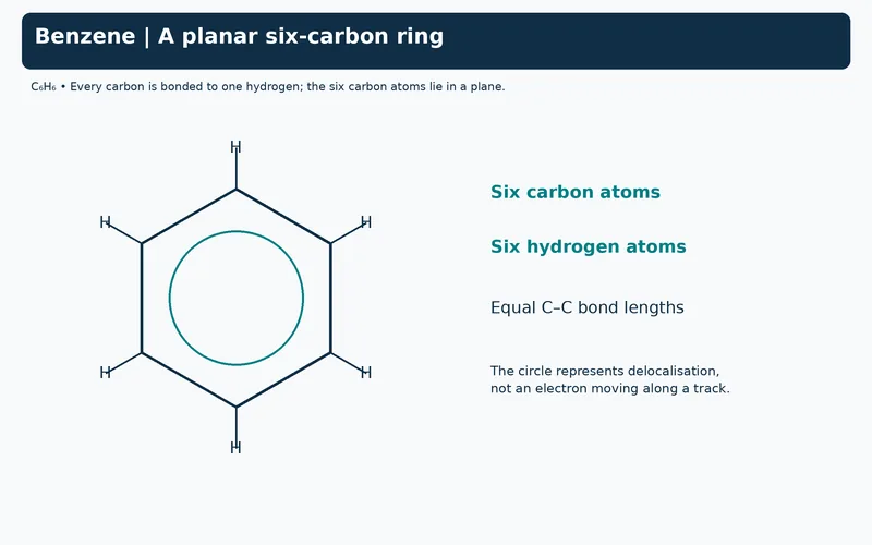 CHEMISTRY · 5 VISUALSBenzene and delocalized electronsBenzene has a planar carbon ring and a delocalised pi system. Resonance drawings are alternative contributors, not separate molecules switching back and forth.
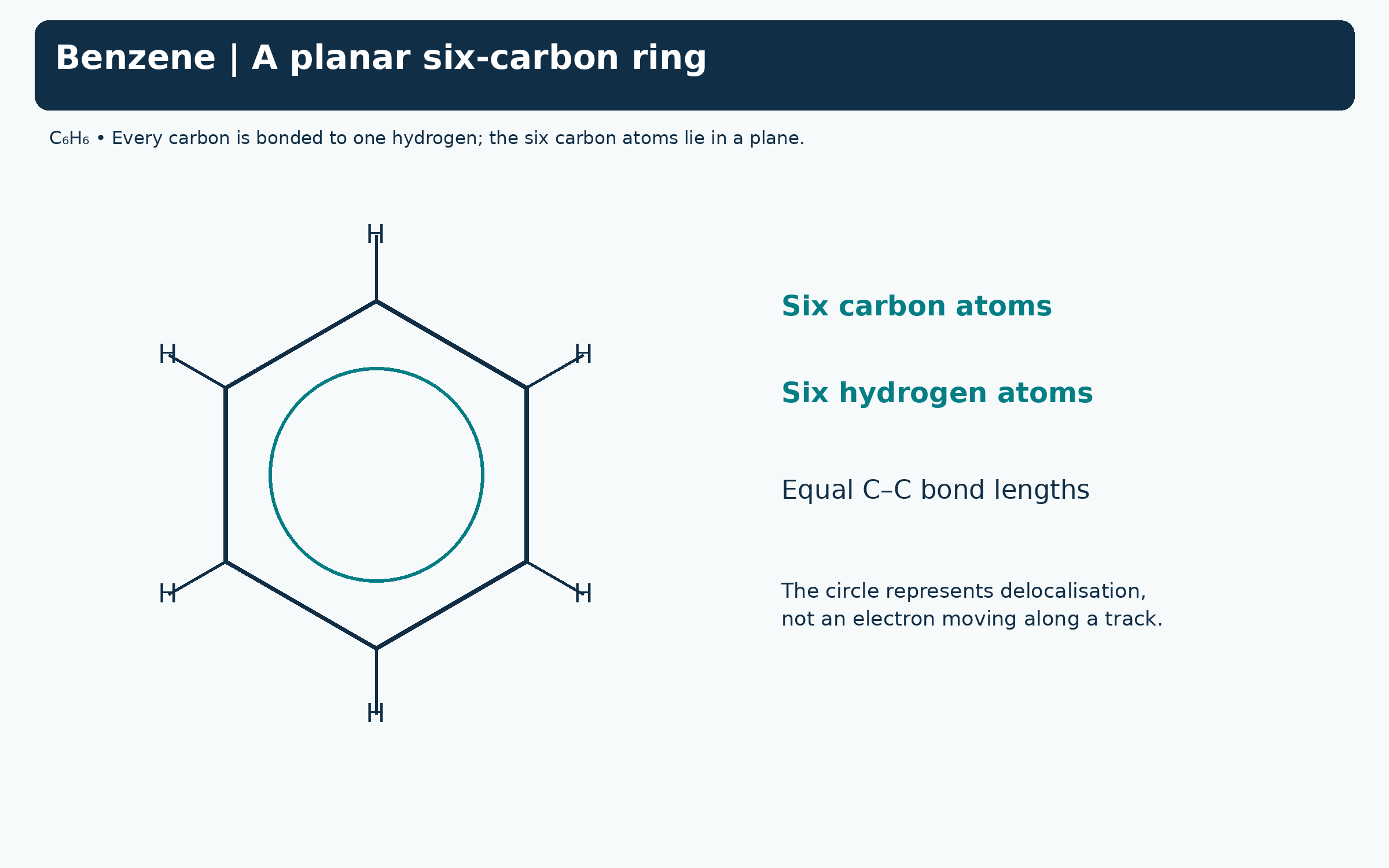
A planar six-carbon ring
A benzene formula shows six carbons, six hydrogens and a circle representing delocalisation.

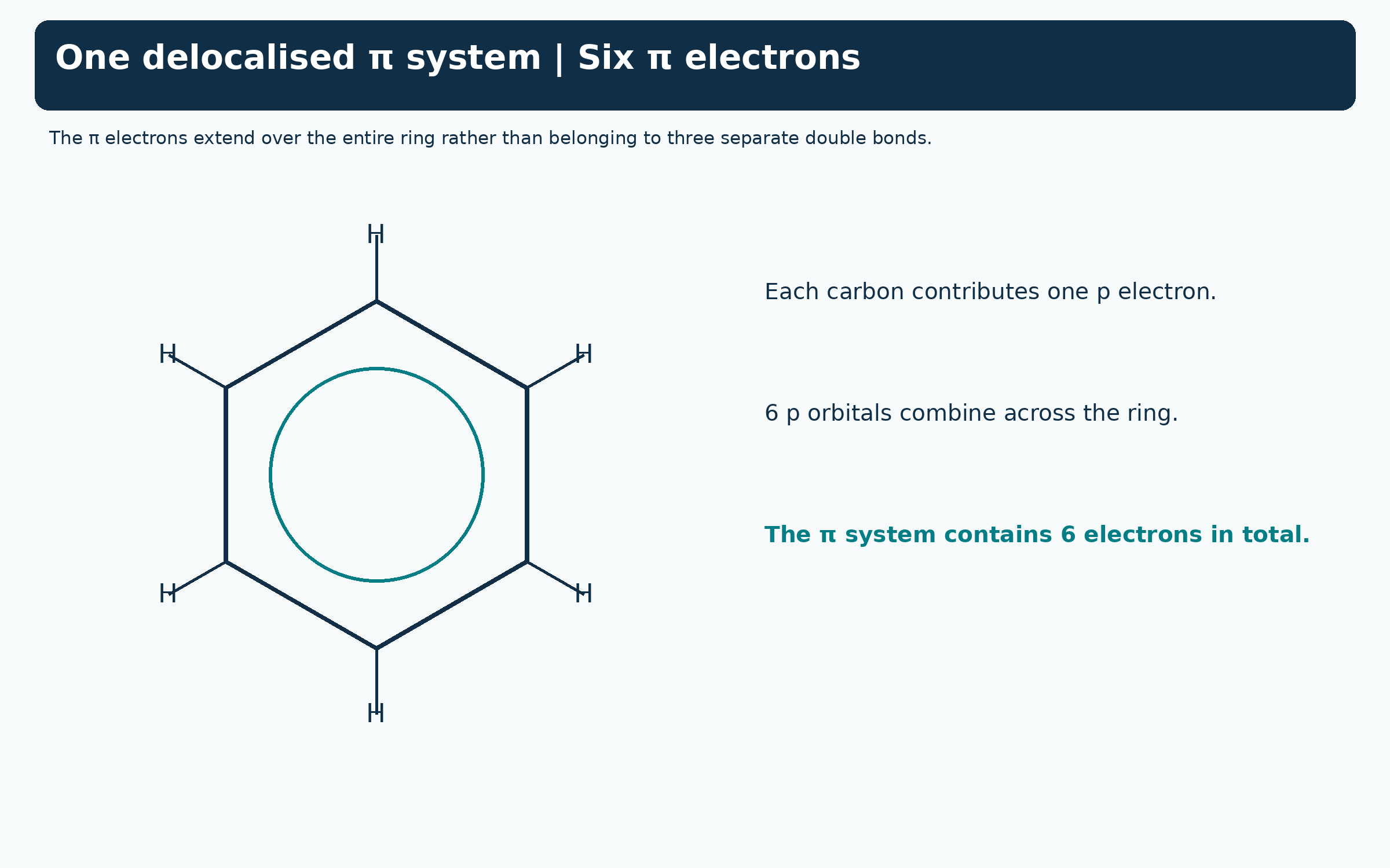
Six electrons in one pi system
The benzene ring is linked to six p orbitals and six delocalised pi electrons.

Kekule contributors
Two alternating-bond drawings are compared with the single delocalised-ring representation.


The pi system above and below the ring
An MMFF-optimised benzene model has schematic translucent pi regions above and below its plane.


Bromination: benzene and ethene
Equations contrast FeBr3-catalysed aromatic substitution with addition across ethene C=C.

 CHEMISTRY · 5 VISUALSCarbonyl geometry and polarityA carbonyl combines trigonal planar geometry with a polar C=O bond. Formaldehyde illustrates how nucleophilic addition changes the carbon geometry.
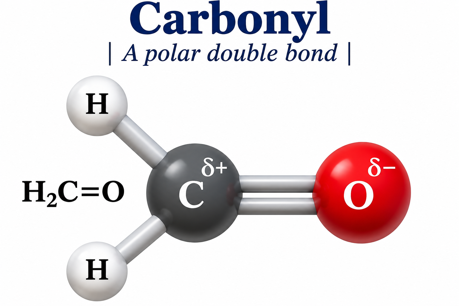
A polar carbonyl bond
Formaldehyde is shown with partially positive carbon and partially negative oxygen.
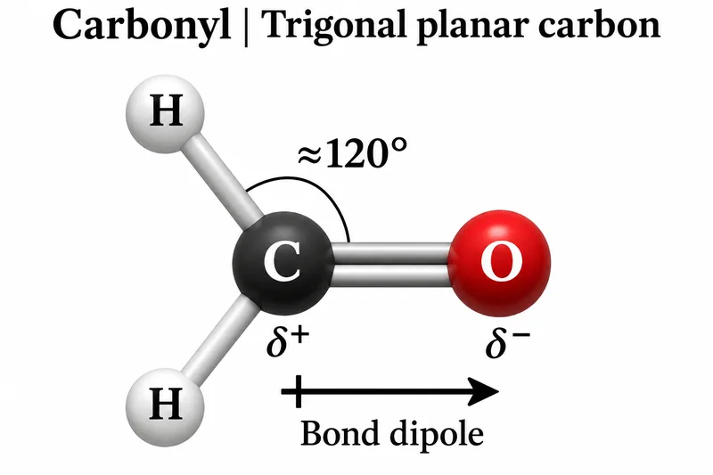
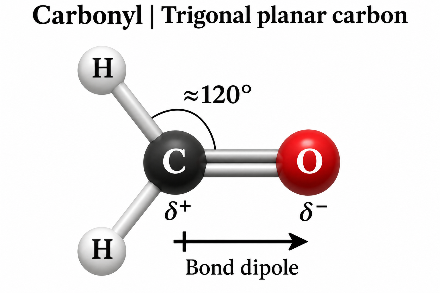
Trigonal planar carbon
A formaldehyde model shows an approximately 120-degree angle and a bond dipole towards oxygen.

Sigma and pi components
A schematic orbital model separates the sigma framework from pi overlap above and below the molecular plane.


Electron-pair arrows in addition
One arrow runs from the nucleophile lone pair to carbon; another moves the C=O pi pair to oxygen.


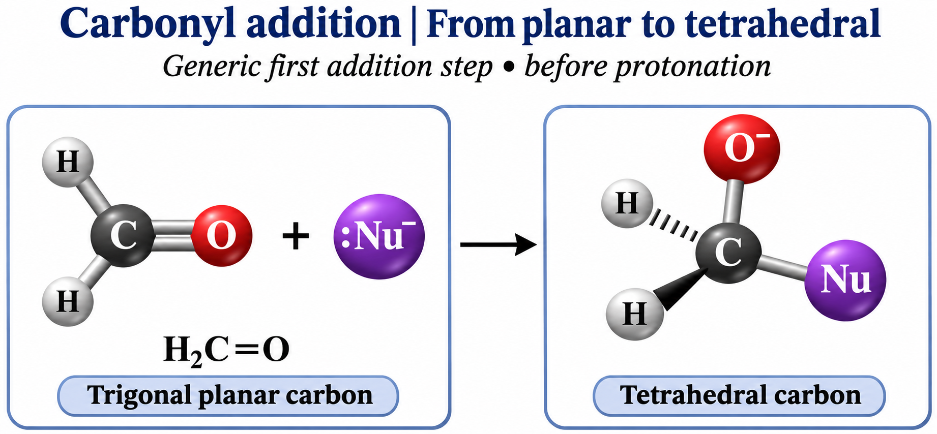
Planar to tetrahedral
A generic nucleophilic addition step gives tetrahedral carbon and negatively charged oxygen before protonation.
 CHEMISTRY · 5 VISUALSElectroplating with copperCopper electroplating deposits copper on the negative electrode. A soluble copper anode supplies copper ions as it is oxidised.
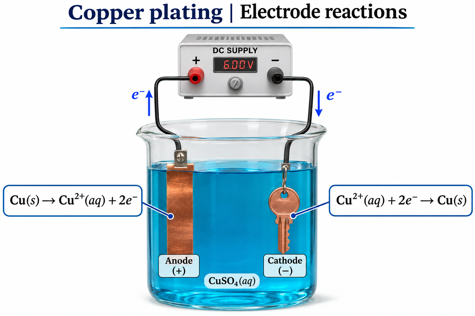
Copper plating apparatus
A copper anode and object cathode sit in copper-ion solution connected to a DC supply.


Copper deposits on the object
Copper ions gain electrons at the negative cathode, illustrated by a plated key.


The electrode half-equations
Copper oxidation at the anode and copper-ion reduction at the cathode accompany external electron arrows.

Electrode mass changes
Before-and-after views show equal copper mass lost and gained under ideal conditions without side reactions.


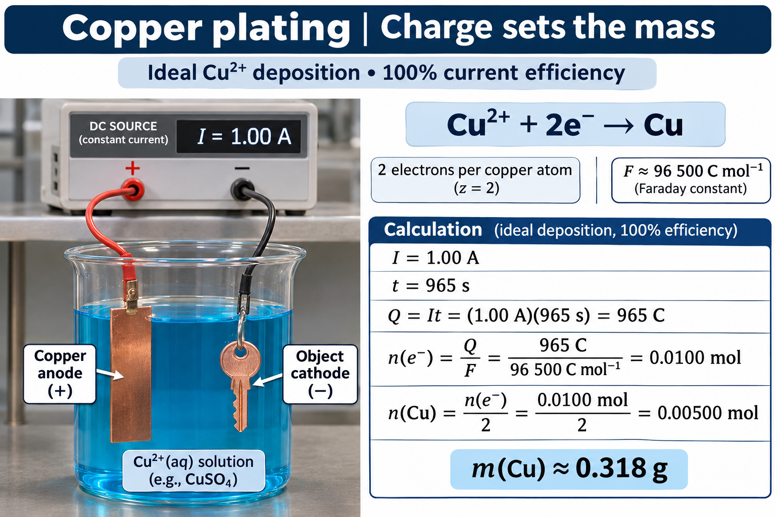
Charge determines deposited mass
An ideal 1.00 A current for 965 s deposits approximately 0.318 g copper at 100 percent current efficiency.
 CHEMISTRY · 5 VISUALSHeterogeneous catalysisA heterogeneous catalyst offers a surface where reactants can adsorb and react. Desorption releases products and leaves sites available again.
Reactants adsorb on a surface
Generic A2 and B2 reactants approach and bind to a catalyst surface.


Three stages of surface catalysis
Adsorption, surface reaction and desorption illustrate the generic equation A2 + B2 → 2AB.

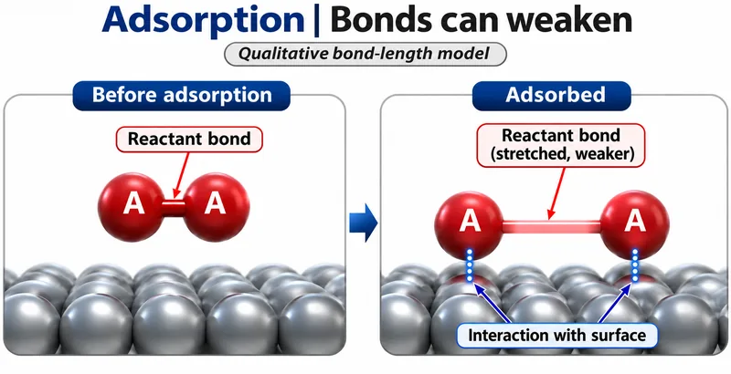
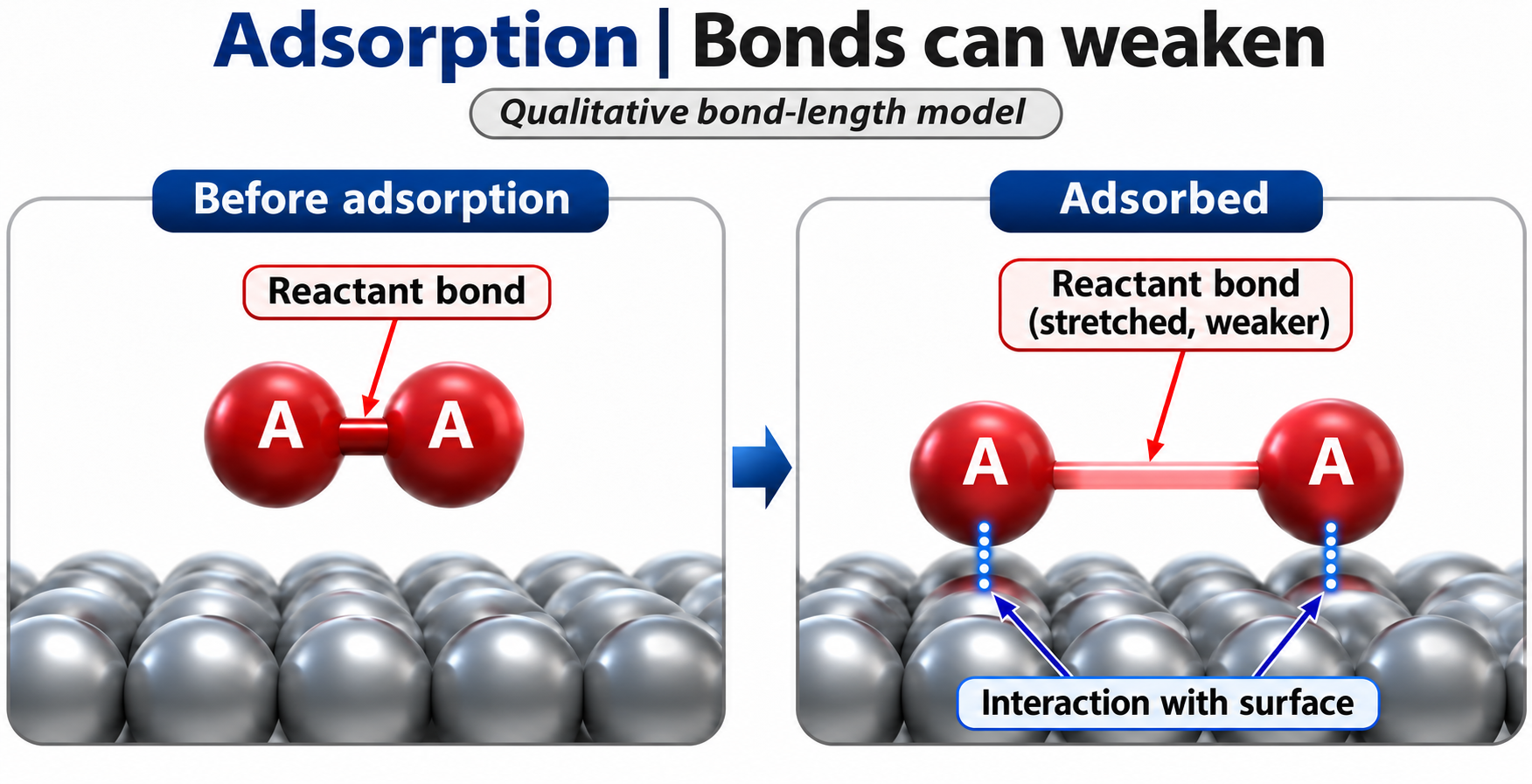
Adsorption can weaken bonds
A qualitative model compares a reactant bond before and after interaction with the surface.

Desorption frees catalytic sites
A surface-bound AB product leaves, making sites available again.

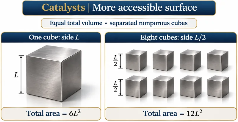
Equal volume, greater surface area
One nonporous cube is compared with eight separated half-side cubes, doubling total surface area.

 CHEMISTRY · 5 VISUALSChoosing a titration indicatorAn indicator changes colour over a pH range, not at one exact value. A suitable range lies within the steep part of the titration curve.
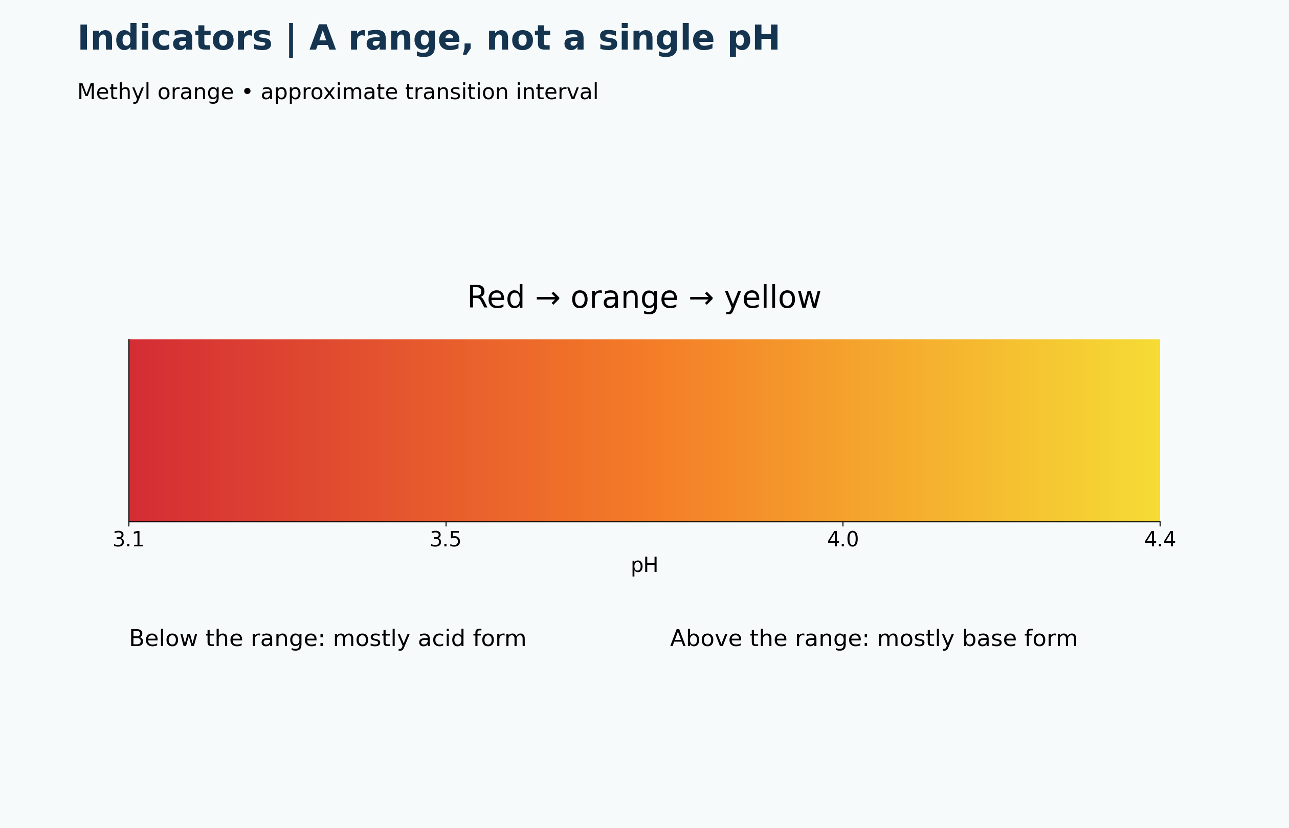
An indicator transition range
Methyl orange changes from red through orange to yellow over an approximate pH range 3.1–4.4.

Matching the steep rise
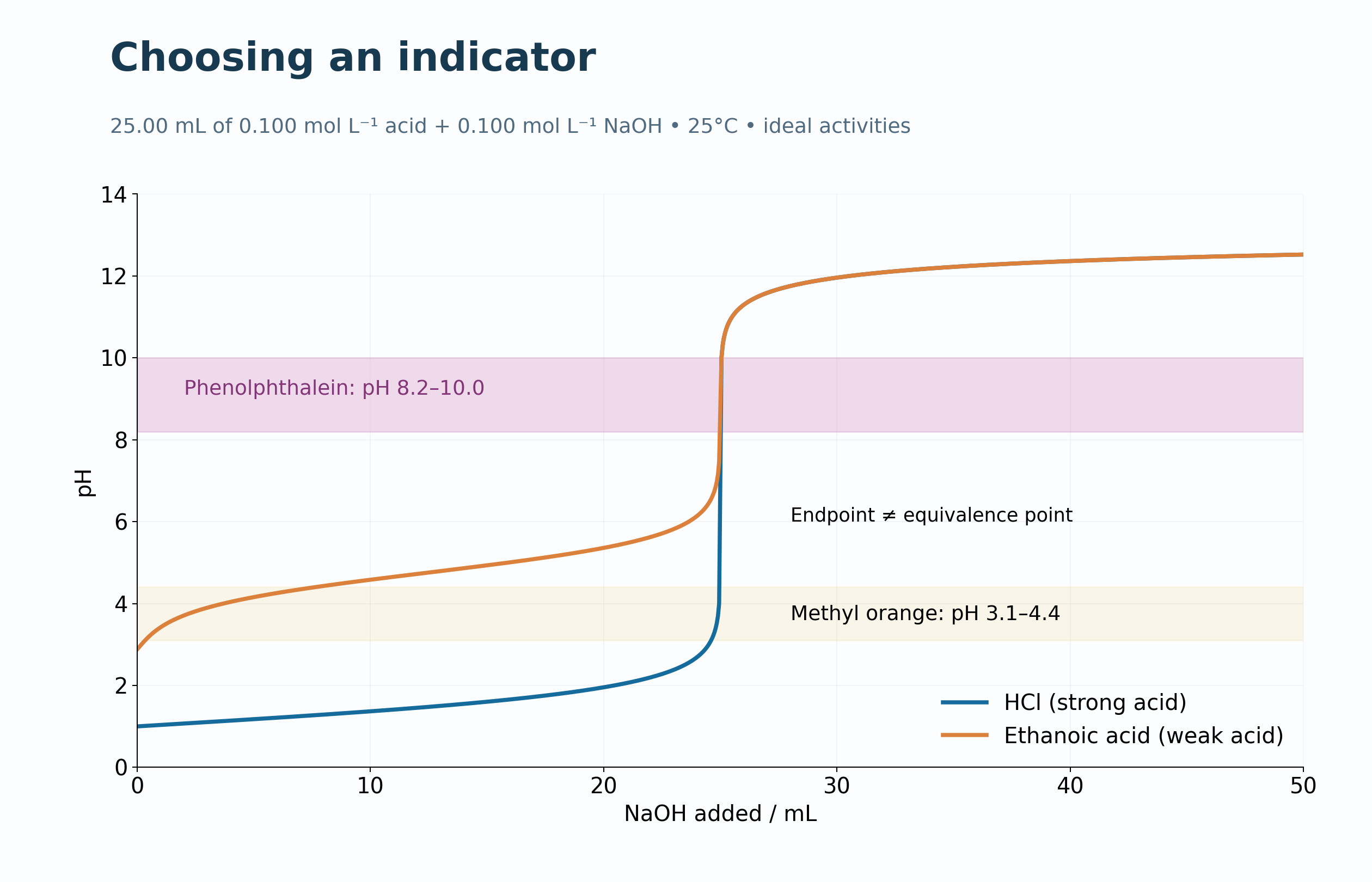
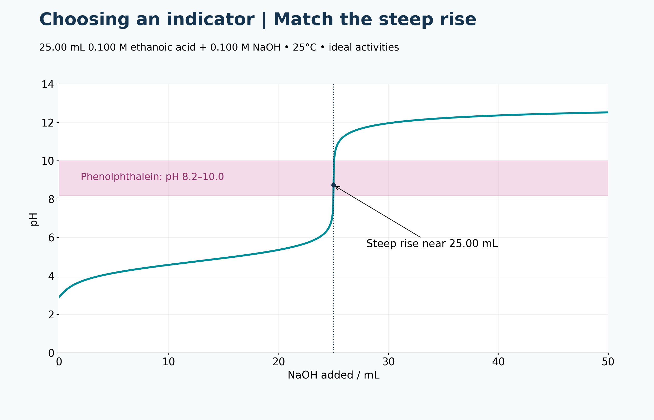
A calculated ethanoic acid–NaOH curve places the phenolphthalein interval around the steep rise near 25.00 mL.

Two coloured indicator forms
A generic HIn equilibrium and concentration-ratio equation connect pH with acid-form and base-form colour.


Comparing two indicators
Phenolphthalein overlaps the steep rise of a weak-acid titration; methyl orange changes colour too early.


Endpoint is not equivalence
The curve distinguishes observed colour change from stoichiometric equivalence at approximately pH 8.73.

 CHEMISTRY · 5 VISUALSHaber process equilibrium and recyclingThe Haber process balances equilibrium yield, reaction rate and energy costs. Cooling removes ammonia while unreacted nitrogen and hydrogen are recycled.
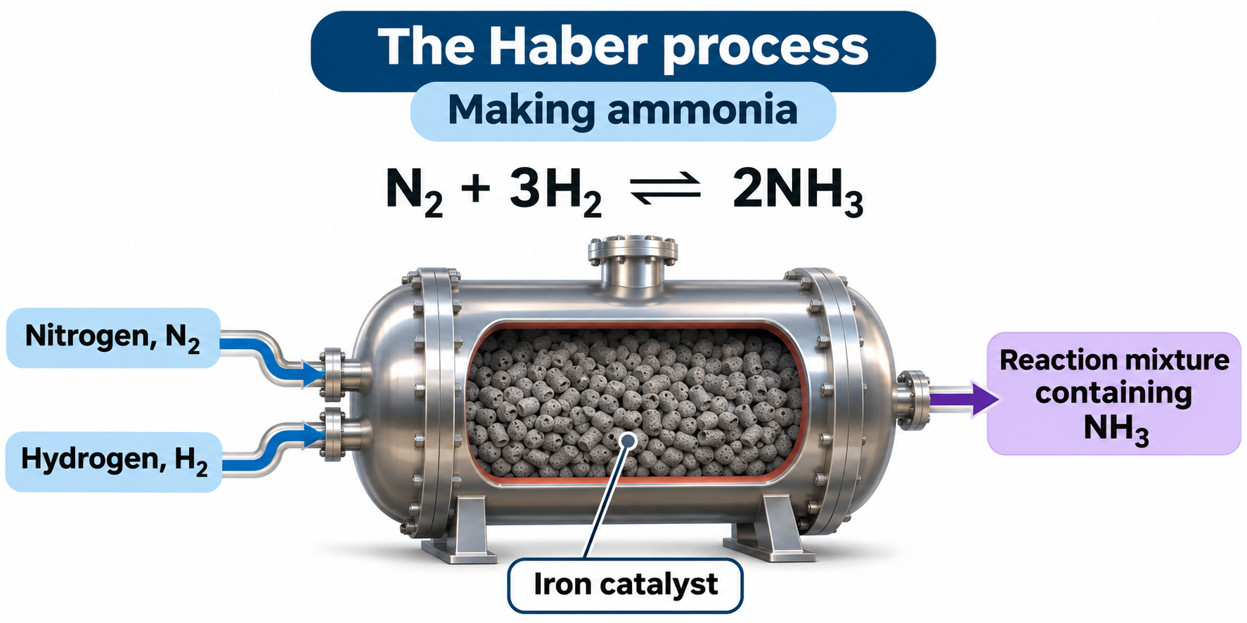
Making ammonia
Nitrogen and hydrogen enter an iron-catalyst reactor, illustrating N2 + 3H2 ⇌ 2NH3.

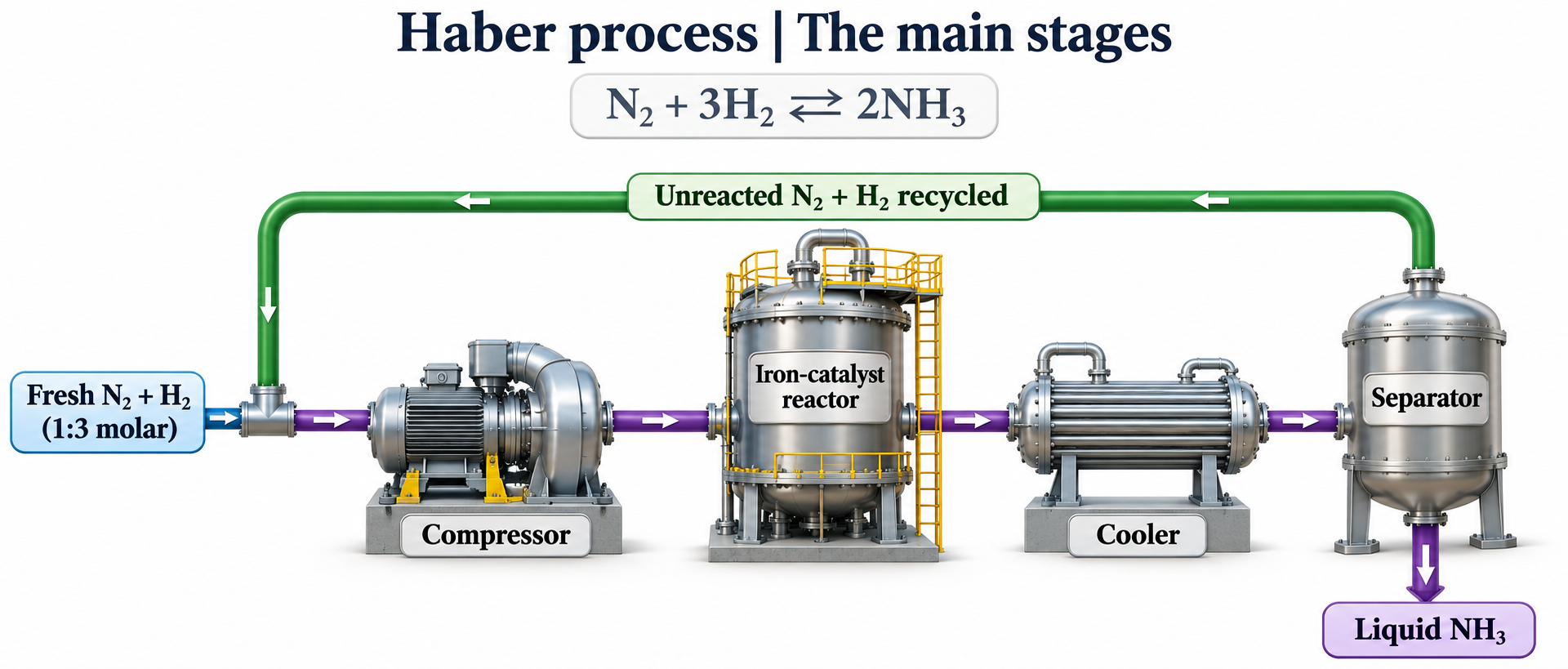
The main process stages
A simplified flow links feed, compressor, reactor, cooler and separator with unreacted-gas recycling.

Yield compared with speed
Pressure, temperature and catalyst panels compare equilibrium and rate effects for ammonia formation.

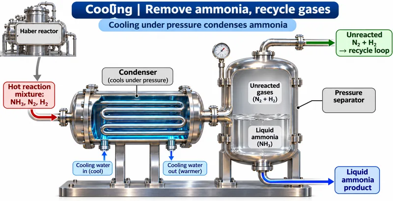
Cooling separates ammonia
A condenser and separator remove liquid ammonia while nitrogen and hydrogen return to the recycle loop.


Recycling with a purge
A simplified industrial flow includes product removal, recycled reactants and a small purge for accumulating inert gases.

 PHYSICS · 5 VISUALSFree-body diagram on an inclineResolve forces on a slope without counting weight components as extra forces.
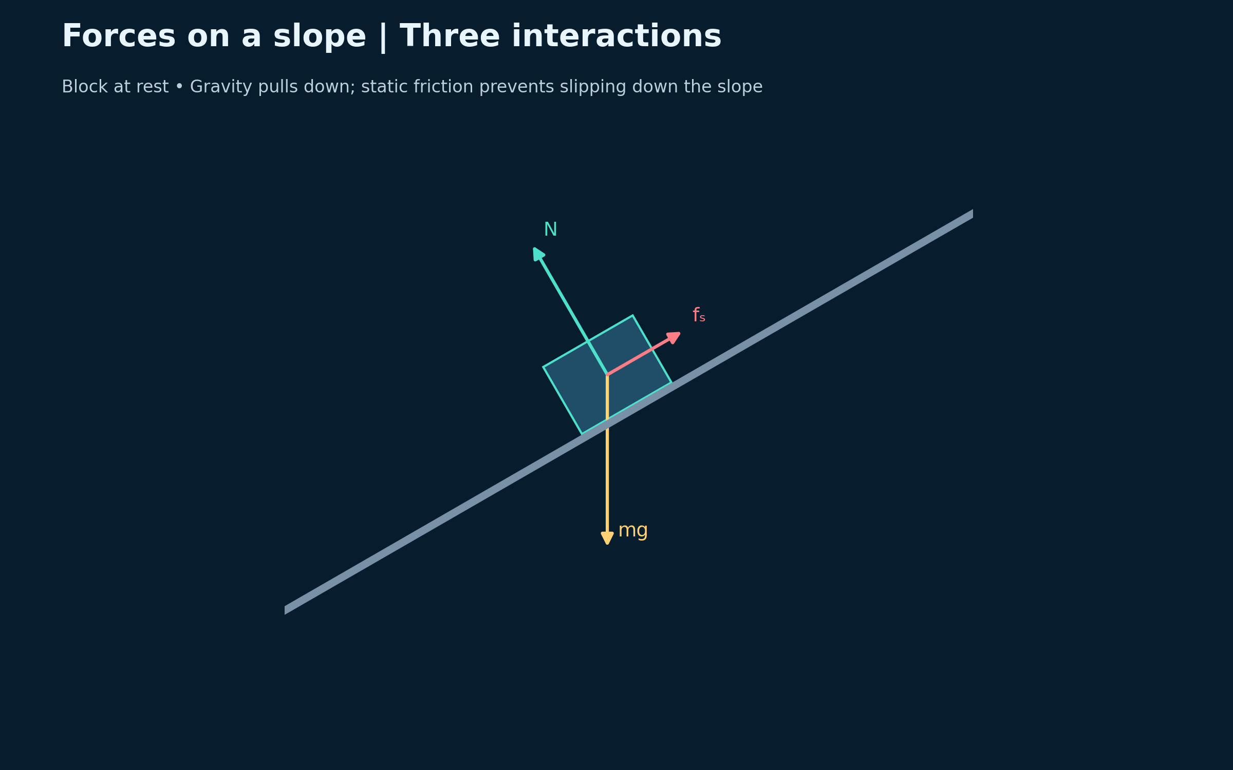
Three forces on a resting block
Weight acts vertically down, the normal force is perpendicular to the slope, and static friction acts uphill.
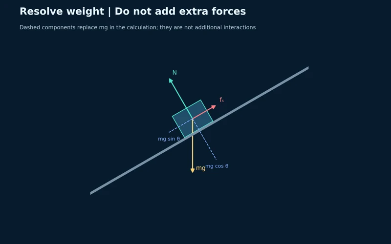
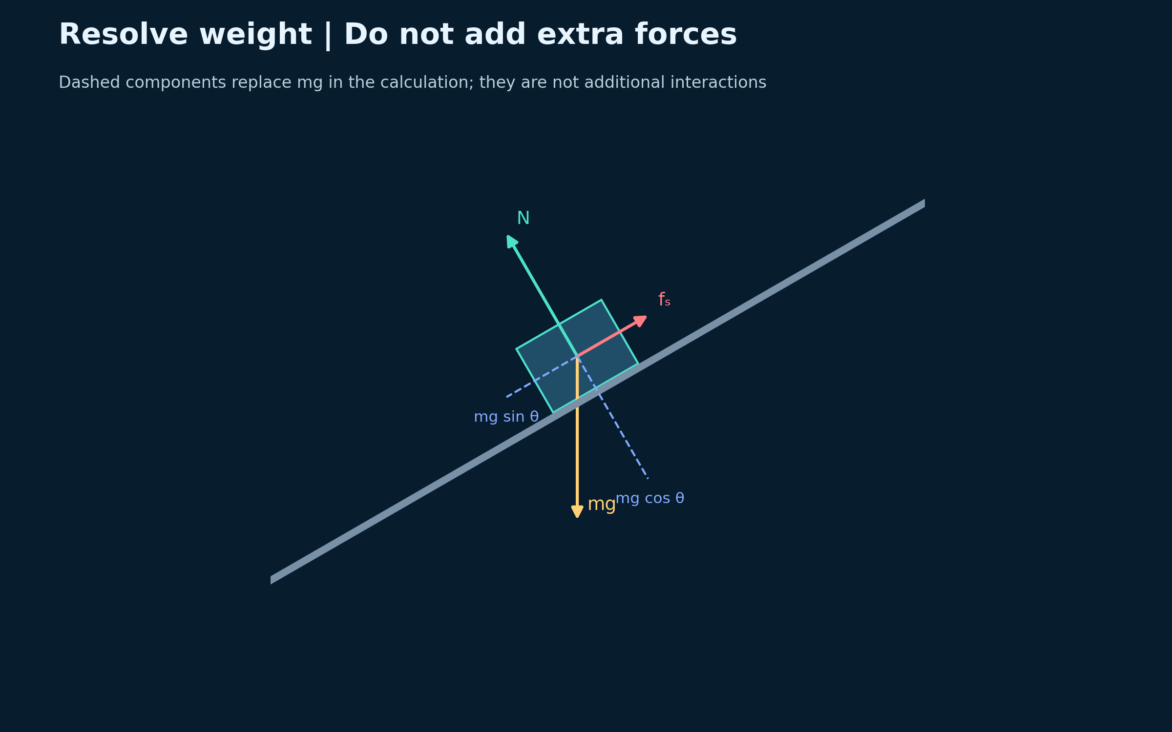
Resolving weight
Dashed components resolve weight parallel and perpendicular to the slope without adding new interactions.

Static and kinetic friction
A 30-degree slope compares adjustable static friction, limiting friction and sliding friction.


Friction opposes relative sliding
Matched diagrams compare a block sliding down and up the same rough slope.


A numerical incline example
A 2.0 kg block on a 30-degree slope has a 6.41 N downhill resultant and acceleration of 3.21 m/s².
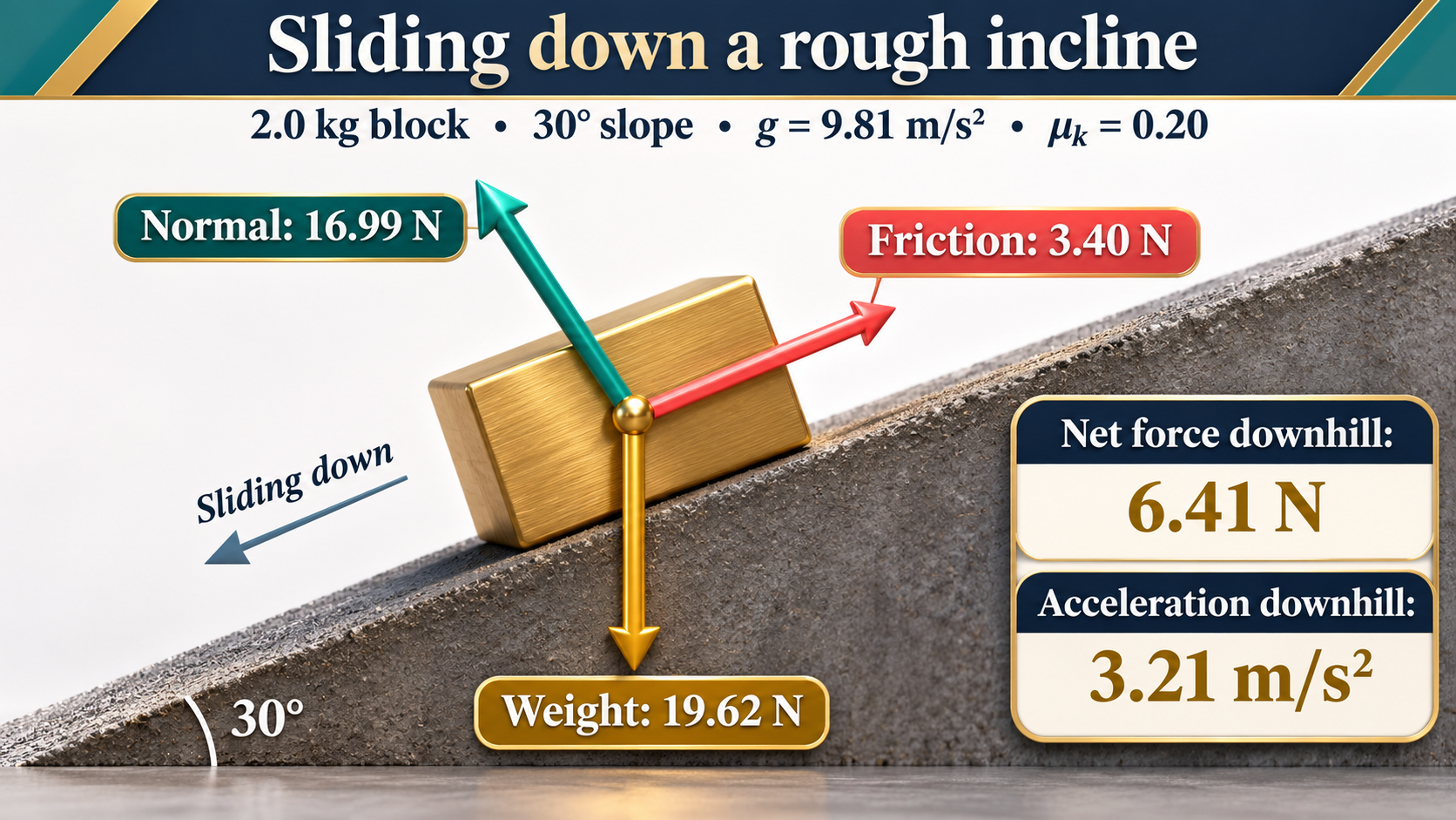
Ideal Newtonian force diagrams on a 30-degree incline. The numerical example uses g = 9.81 m/s² and kinetic friction coefficient 0.20. The apparatus scene is an illustration, not a measured experiment.
 PHYSICS · 5 VISUALSProjectile motion: independent componentsConnect a projectile trajectory with independent horizontal and vertical motion.
Equal times on a parabolic path
Half-second markers show a projectile launched and landing at the same height with air resistance neglected.


Independent velocity components
Horizontal velocity stays at 12 m/s while vertical velocity changes under gravity.


Two equations, one time
The example x = 12t and y = 15t − 5t² gives a 3.0 s flight, 36 m range and 11.25 m maximum height.


Complementary launch angles
Equal-speed launches at 30 and 60 degrees have the same range but different heights and flight times.

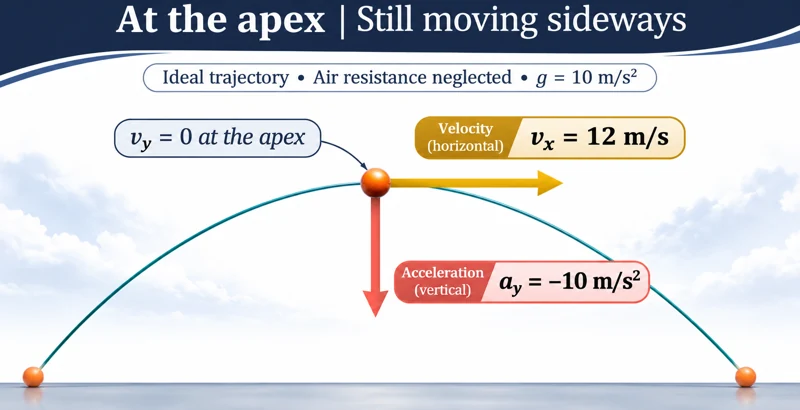
Motion at the apex
At the apex, vertical velocity is zero while horizontal velocity and downward acceleration remain nonzero.
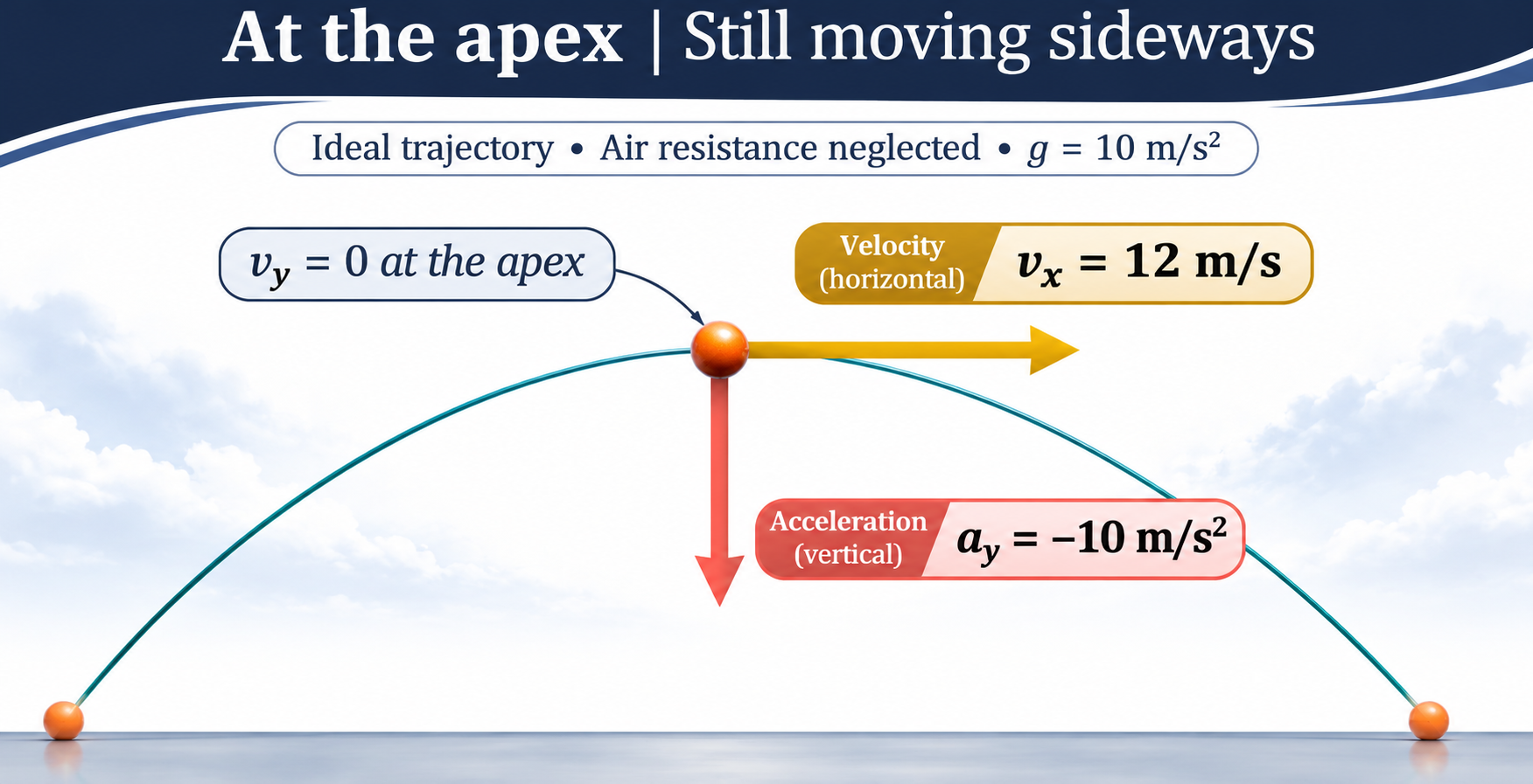
Ideal near-Earth projectile model with no air resistance, g = 10 m/s², and equal launch and landing heights. The apex scene is illustrative rather than a calibrated photograph.
 PHYSICS · 5 VISUALSVector addition, head-to-tailAdd, resolve and subtract vectors using consistent Cartesian components.
Head-to-tail addition
Vectors A = (4, 1) N and B = (1, 3) N join head-to-tail to form their resultant.

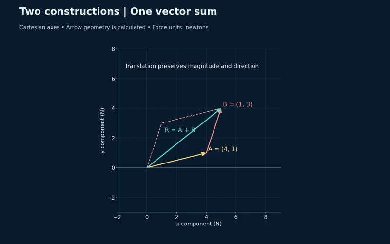
Two equivalent constructions
A parallelogram and a head-to-tail construction give the same vector sum.

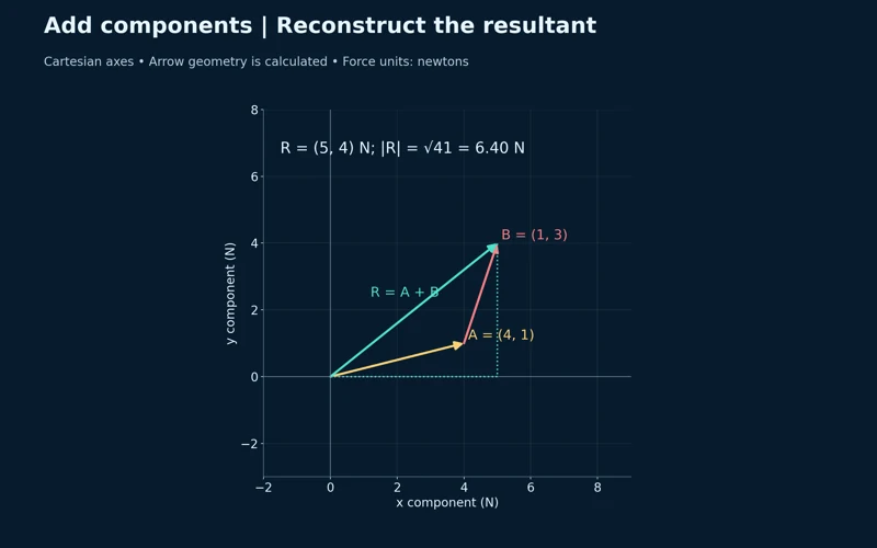
Adding components
The resultant (5, 4) N has magnitude approximately 6.40 N.

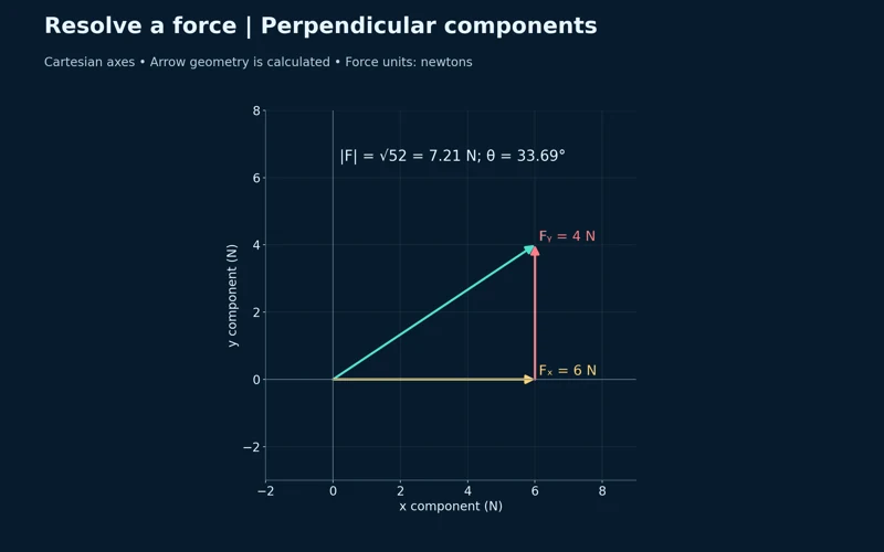
Resolving a force
Perpendicular components of 6 N and 4 N reconstruct a force of approximately 7.21 N.
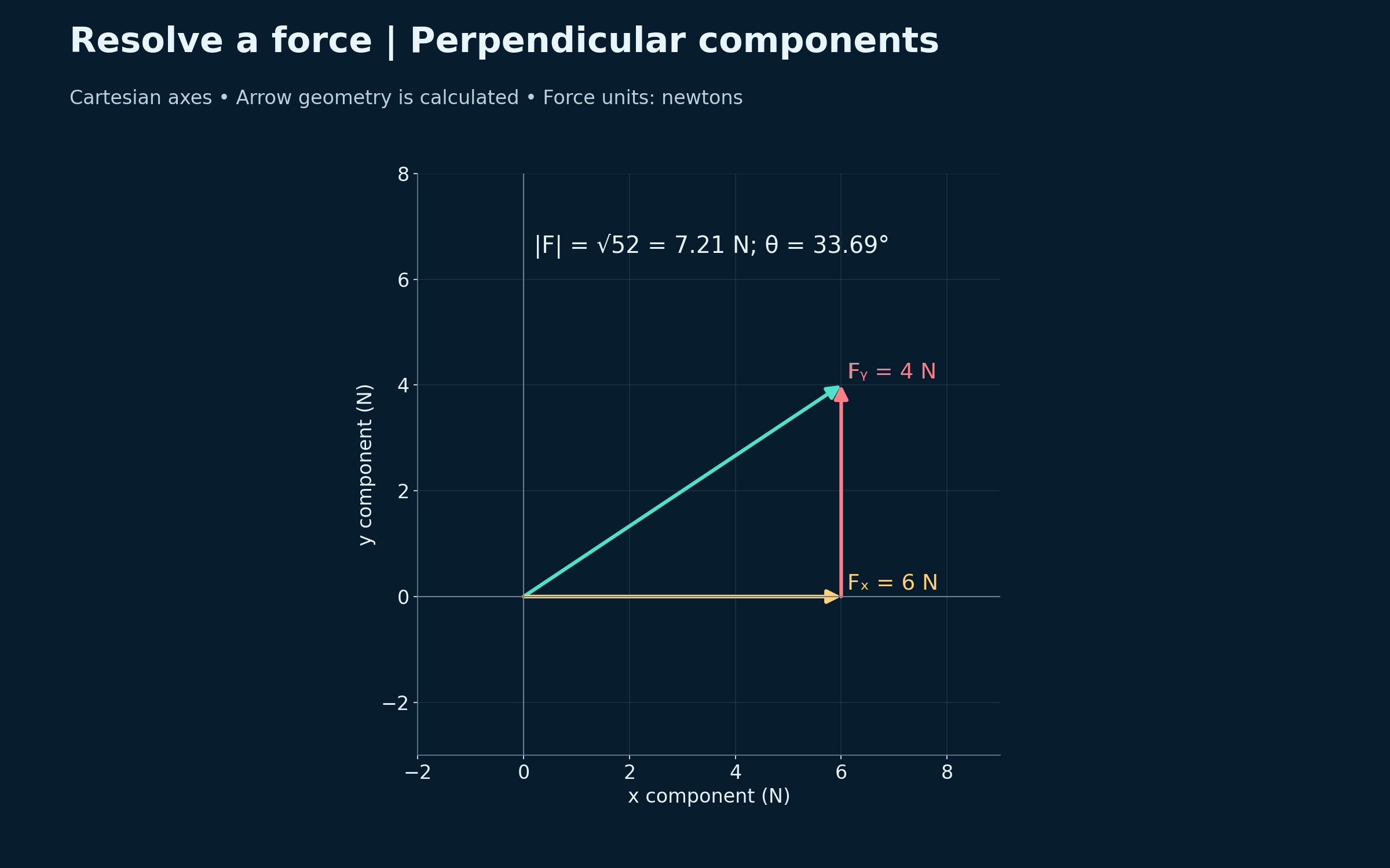

Subtracting a vector
Adding the negative of B gives A − B = (3, −2) N, with magnitude approximately 3.61 N.
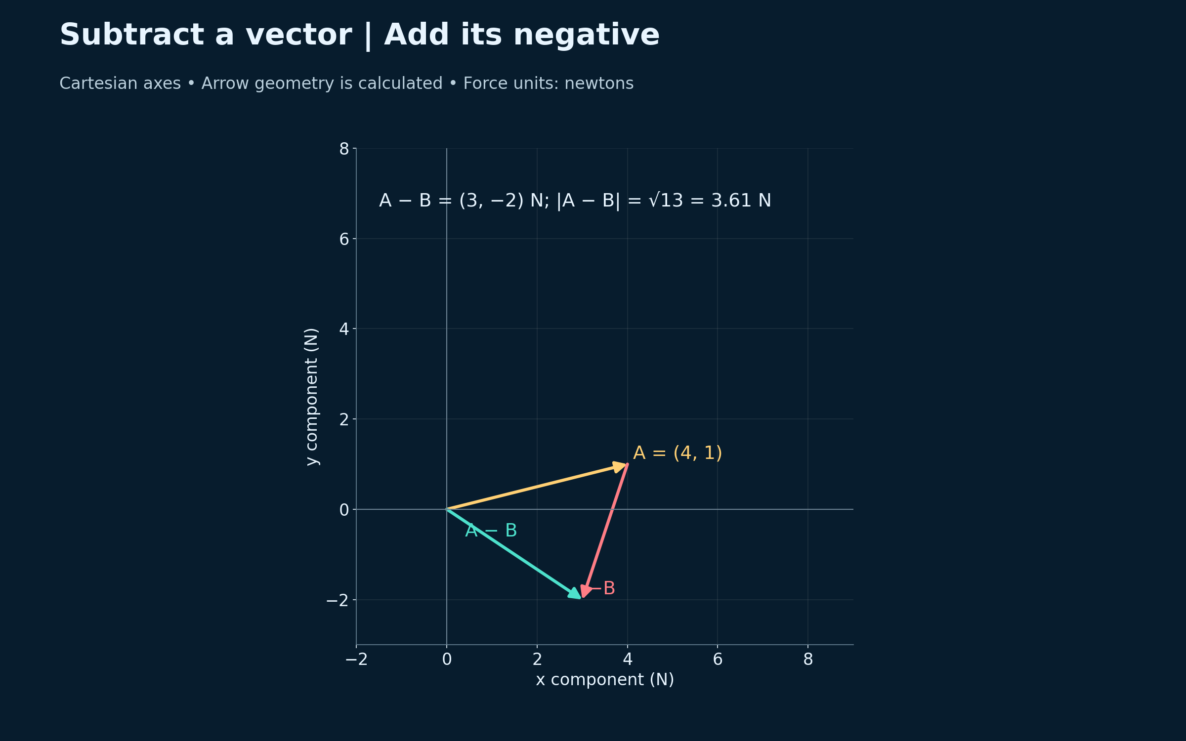
Calculated two-dimensional Cartesian vector geometry. Force components and magnitudes are numerical examples, not measurements.
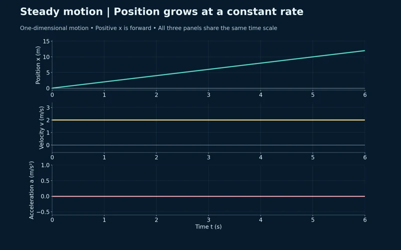 PHYSICS · 5 VISUALSPosition–velocity–acceleration graphsLink position, velocity and acceleration through graph gradients and signed areas.
Steady forward motion
Position increases linearly while velocity remains 2 m/s and acceleration is zero.
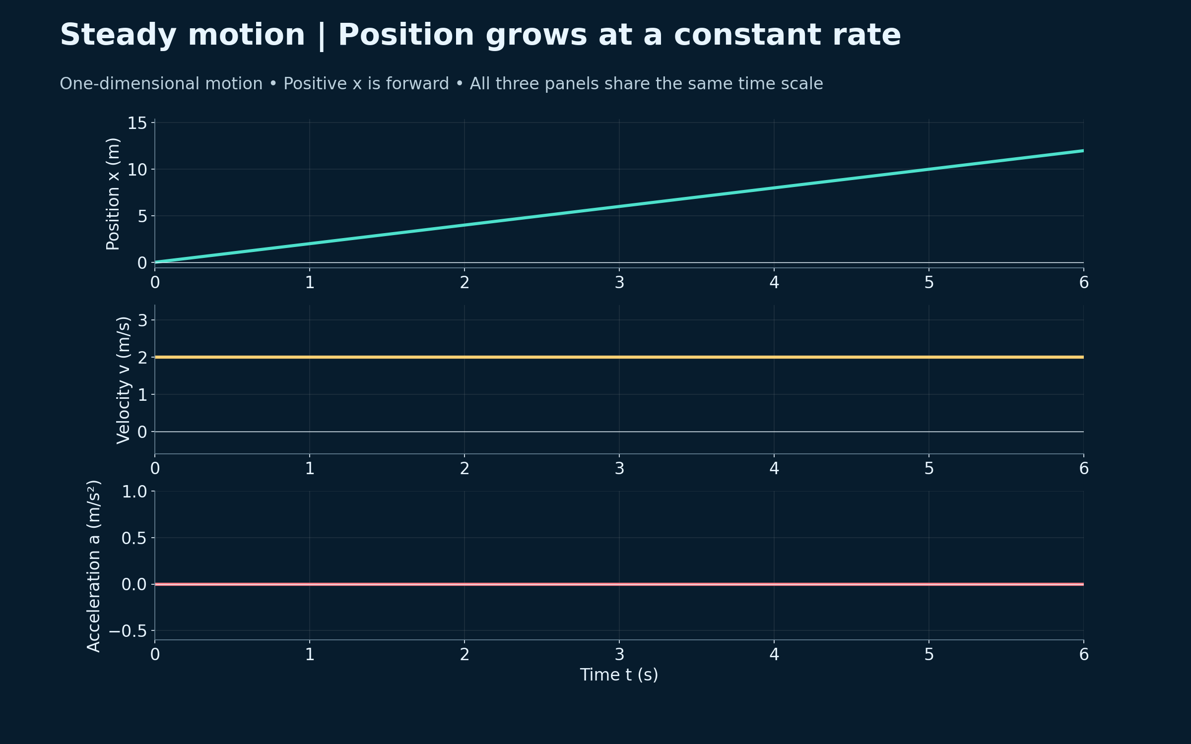

Uniform acceleration
Aligned graphs show x = t², v = 2t and a = 2 m/s².


Gradients link the graphs
Tangents show that the position gradient gives velocity and the velocity gradient gives acceleration.


Signed areas recover changes
Shaded areas from 1 to 3 s give an 8 m displacement and a 4 m/s velocity change.


Speed up, cruise, slow down
A piecewise motion story links accelerating, steady-speed and decelerating intervals across three graphs.

Calculated one-dimensional motion models with shared time axes. The piecewise example idealises instantaneous changes in acceleration.
 PHYSICS · 5 VISUALSNewton third-law interaction pairsSeparate Newton’s third-law force pairs from the forces acting on one object.
Forces on different bodies
Two skaters push each other with equal-magnitude, opposite-direction contact forces.


Separate free-body diagrams
Each skater has its own horizontal contact force, weight and normal force.


Equal forces, unequal accelerations
A 120 N contact force gives 40 kg and 80 kg skaters accelerations of 3.0 and 1.5 m/s².
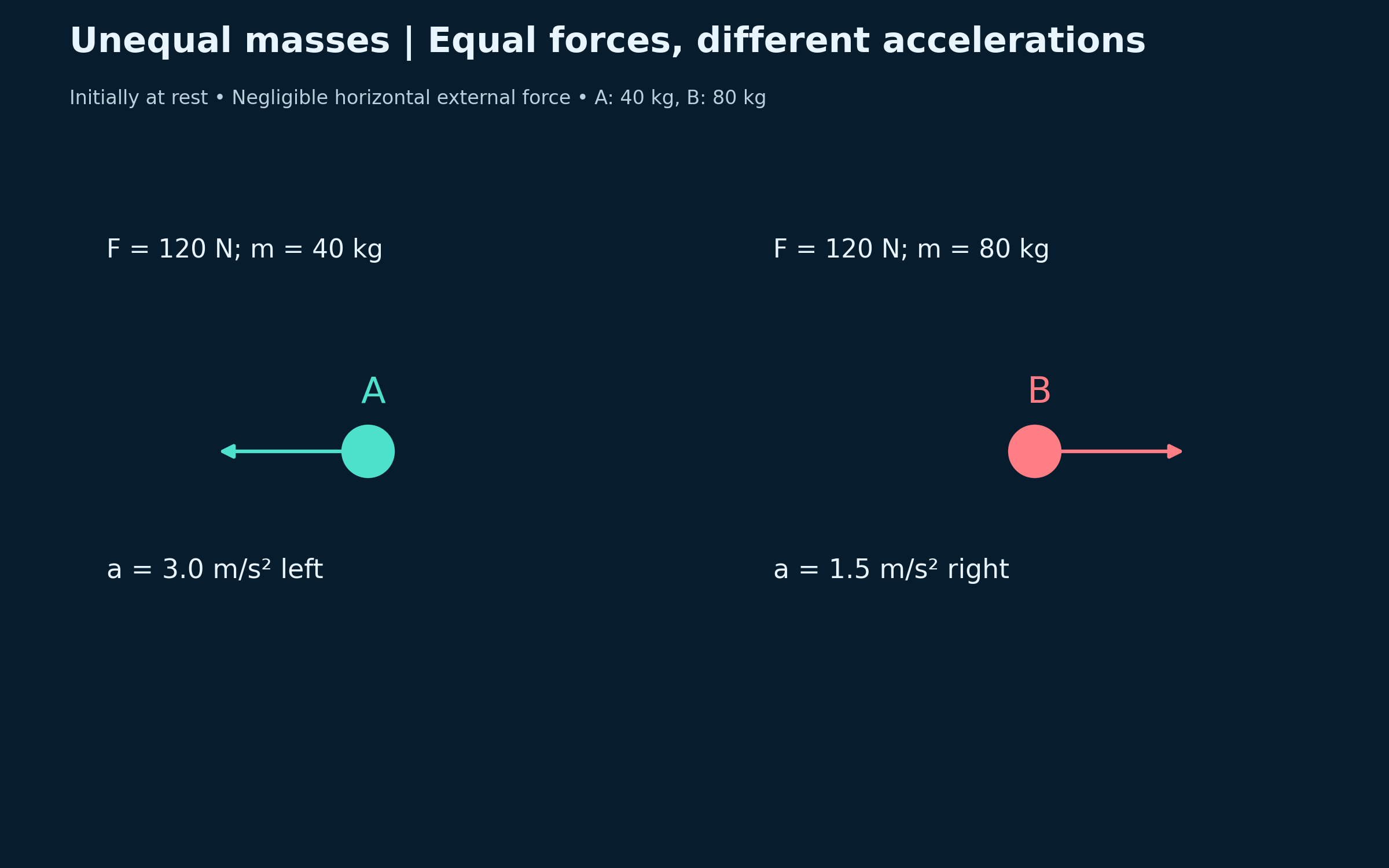

Equal and opposite impulses
A half-second push gives impulses of −60 and +60 N s but different velocity changes.


Momentum of the two-skater system
After the push, equal and opposite momenta give zero total momentum for the initially stationary system.

Ideal two-skater model with negligible external horizontal impulse. Numerical examples use masses 40 kg and 80 kg and equal 120 N contact forces; the scene is illustrative.
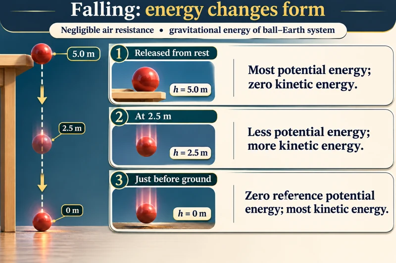 PHYSICS · 5 VISUALSWork and energy transfersTrack energy transfers in falling objects, rough ramps and work calculations.
Falling changes energy stores
A ball released from rest loses gravitational potential energy and gains kinetic energy as it falls.

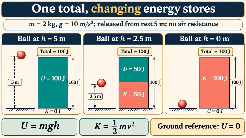
One constant energy total
Energy bars for a 2 kg ball at three heights share a total of 100 J in the stated ideal model.
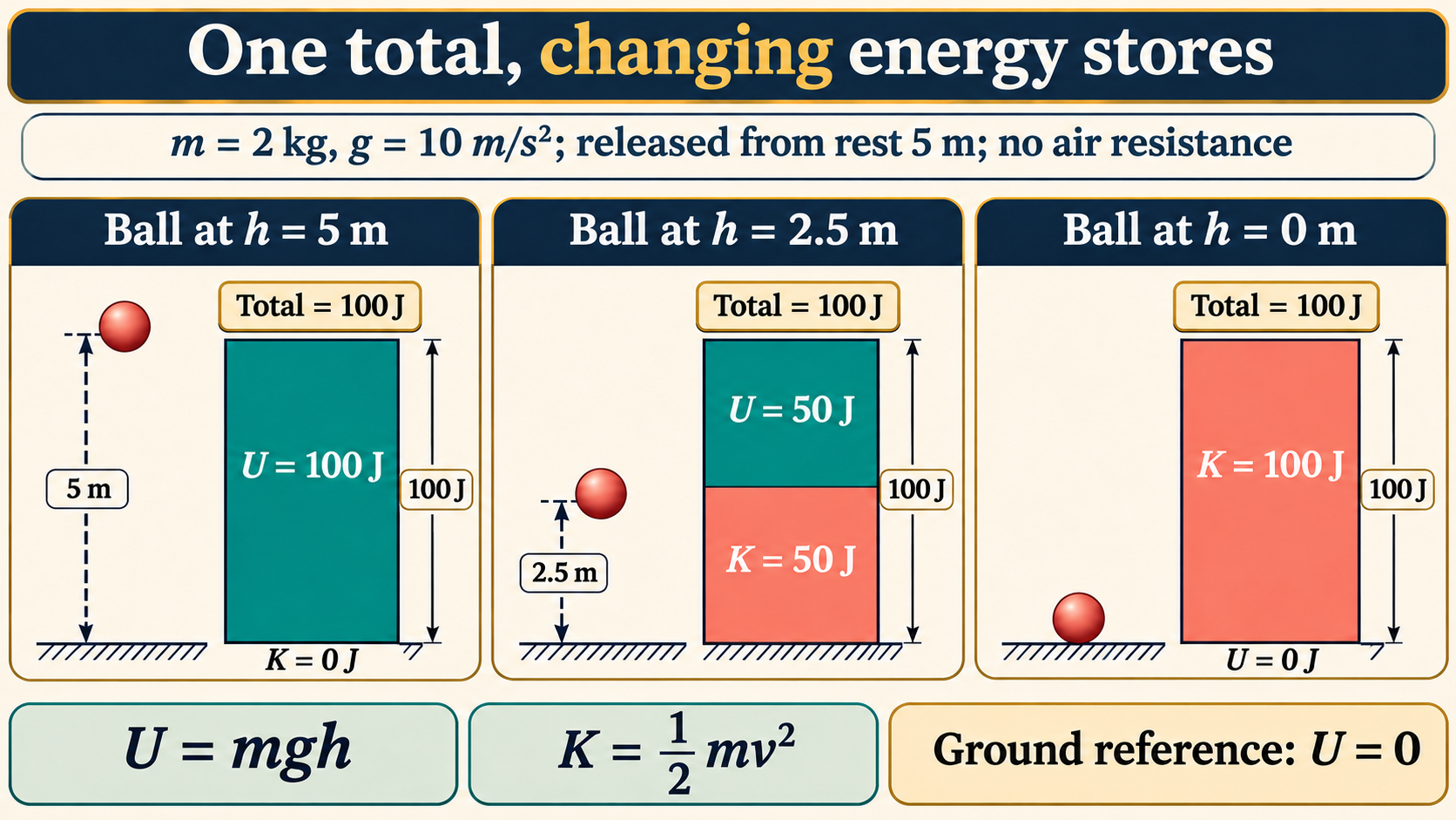
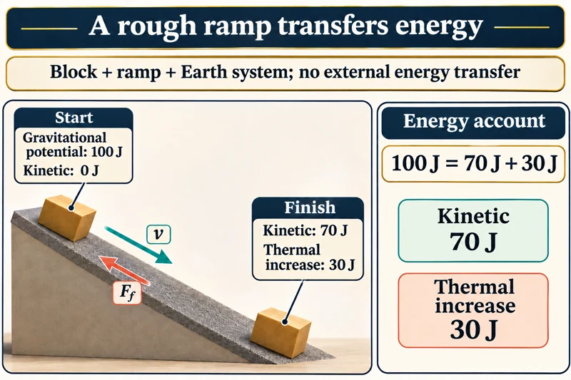
A rough ramp transfers energy
An initial 100 J gravitational store becomes 70 J kinetic energy and a 30 J thermal increase.
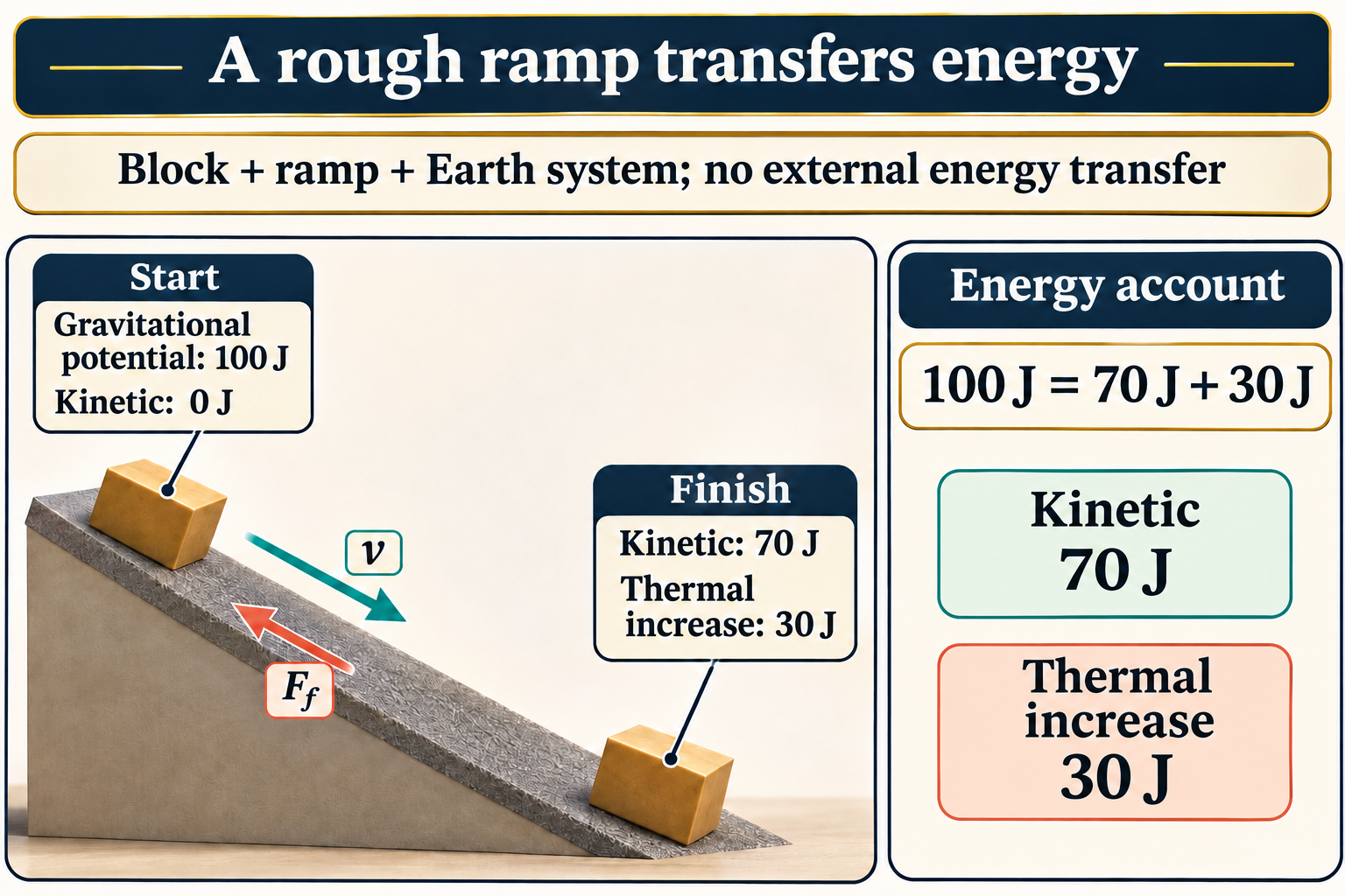
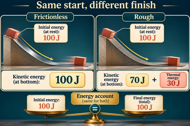
Smooth and rough ramps
Matched ramps compare final energy stores while preserving the same 100 J total.


Net work changes kinetic energy
A 10 N applied force and 4 N friction over 3 m give 18 J net work and an 18 J kinetic-energy increase.

Illustrative energy accounts for explicitly chosen systems. Falling-object calculations neglect air resistance and use g = 10 m/s². Ramp energy values are teaching examples, not measurements.
 PHYSICS · 5 VISUALSMomentum before and after collisionCompare momentum and kinetic energy before and after ideal collisions.
Equal-mass elastic collision
A moving 1 kg cart transfers its 2 m/s velocity to an initially stationary identical cart.


Momentum has a sign
Before-and-after cart diagrams and scaled momentum arrows show the same total momentum of 6 kg m/s.


Checking an elastic collision
A worked unequal-mass collision conserves both 6 kg m/s momentum and 9 J kinetic energy.


Sticking together
Two carts couple at 2 m/s, conserving momentum while 3 J transfers from kinetic to internal energy.

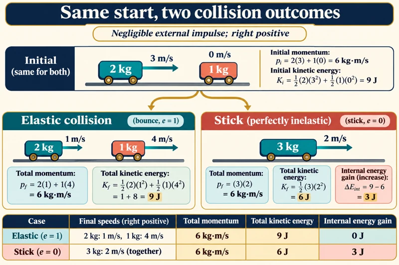
Two outcomes from one start
A side-by-side comparison distinguishes elastic and perfectly inelastic collisions from the same initial conditions.
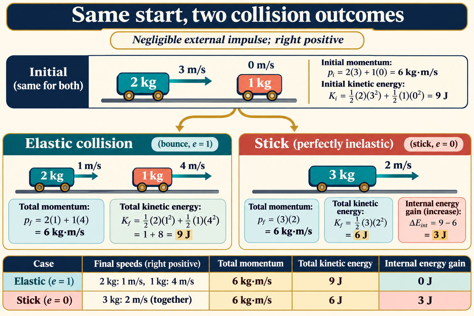
Ideal one-dimensional collision models with negligible external impulse. Elastic and perfectly inelastic cases are limiting models; illustrated carts are not measured apparatus.
 PHYSICS · 5 VISUALSSeries/parallel circuit comparisonCompare current paths, potential differences and power in series and parallel circuits.
One path or two branches
Circuit symbols compare two lamps in series with two lamps connected in parallel.


Current at a junction
Two 6 Ω resistors give 0.5 A in series or two 1 A branches in parallel with a 6 V supply.


Resistance and power
At 6 V, the series combination draws 3 W and the parallel combination draws 12 W.


Opening one lamp
An open series circuit stops both lamps; an intact parallel branch still provides a complete path.
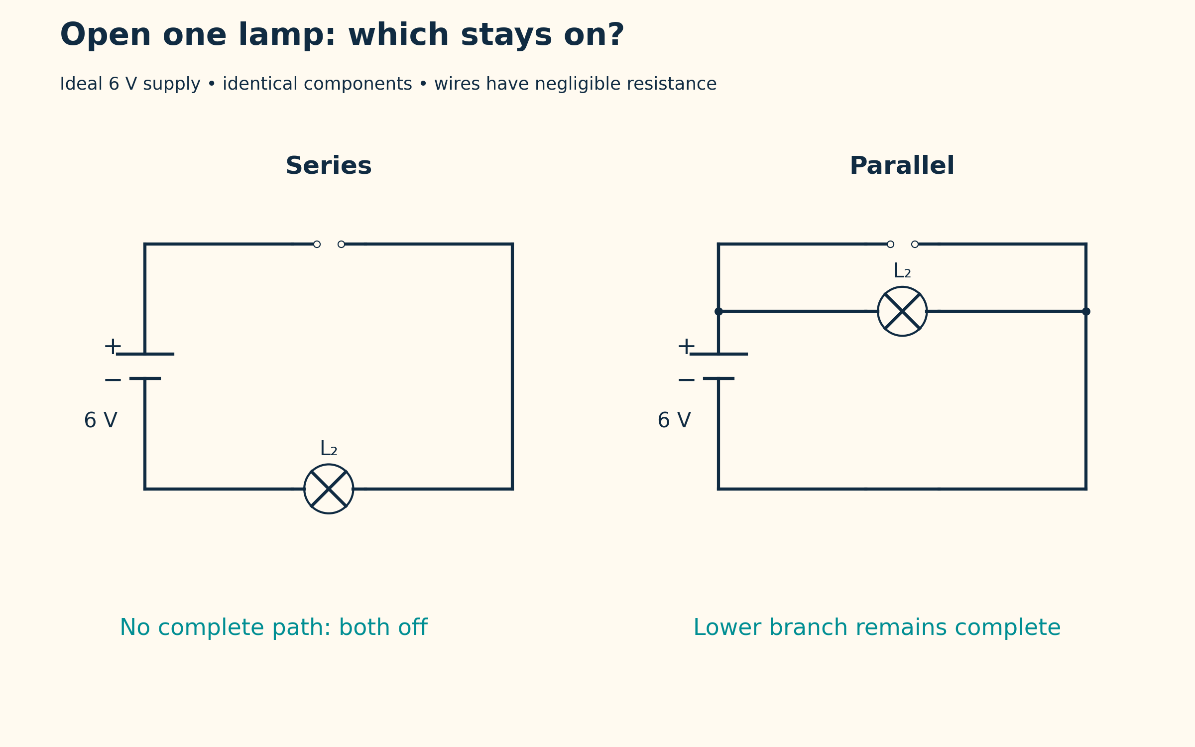

Potential difference across components
Identical series resistors share 6 V, while each parallel branch spans the full supply.

Ideal 6 V source, negligible wire resistance and identical components. Numerical resistor examples use 6 Ω resistors; real lamps need not have constant resistance.
 PHYSICS · 5 VISUALSCurrent, voltage and resistanceDistinguish current, potential difference and resistance with simple circuit models.
Current in a complete circuit
A 6 V supply drives 1 A through a 6 Ω resistor, with conventional current direction indicated.


Connecting the meters
An ammeter is in series and a voltmeter is connected across the resistor.
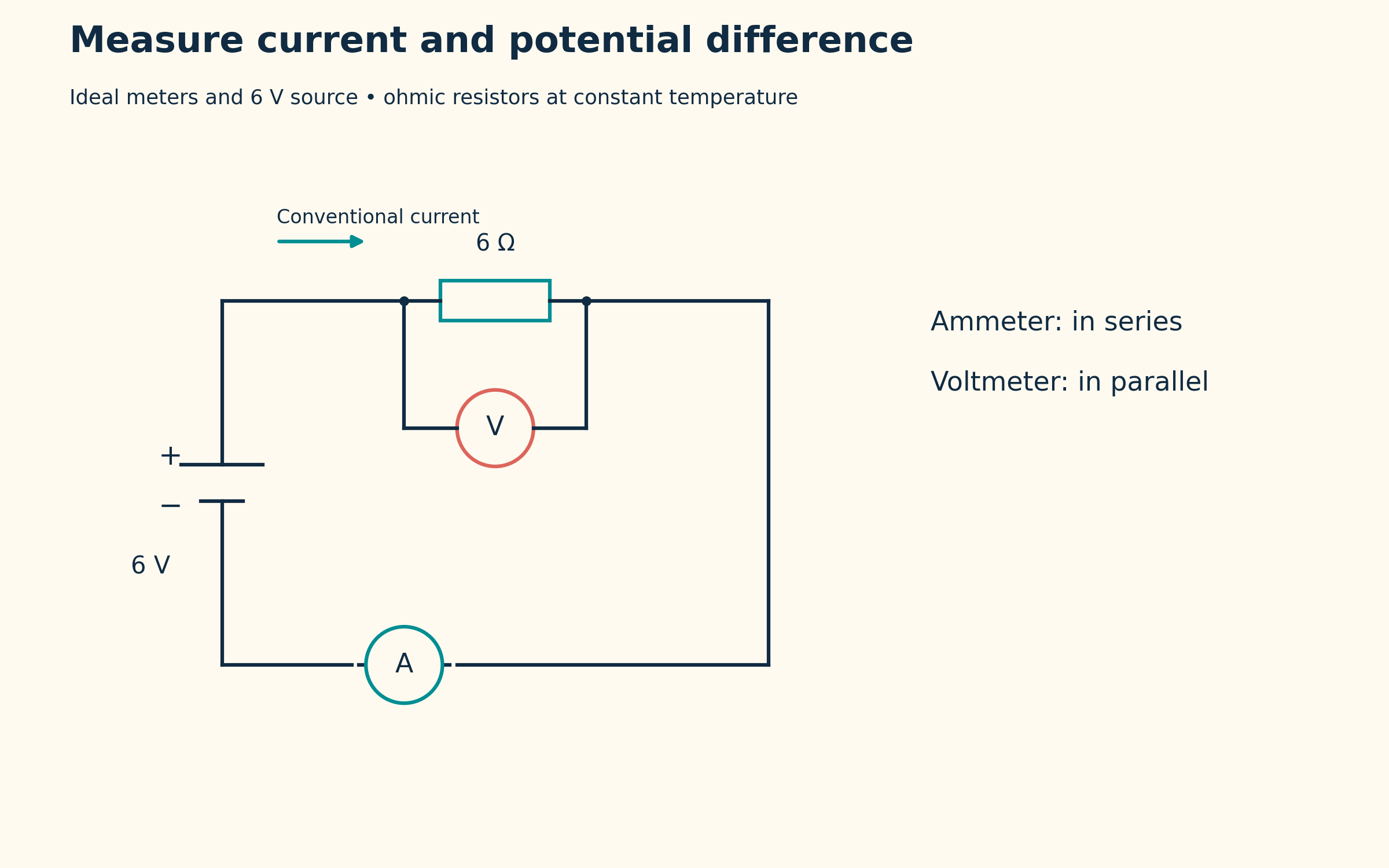

Reading resistance from a graph
A straight potential-difference versus current graph has gradient 6 Ω.


Changing resistance at fixed voltage
A 6 V supply drives 2 A through 3 Ω and 1 A through 6 Ω, with corresponding power values.


Energy transferred per charge
The relation V = W/Q connects 6 V with 6 J/C and a 12 J transfer for 2 C.

Ideal meters and a 6 V source with ohmic resistors at constant temperature. The plotted straight line is a model, not measured data.
 PHYSICS · 5 VISUALSTransverse versus longitudinal wavesDistinguish particle motion from wave propagation in transverse and longitudinal models.
Two kinds of wave motion
Transverse displacement and longitudinal particle positions show motion perpendicular and parallel to propagation.
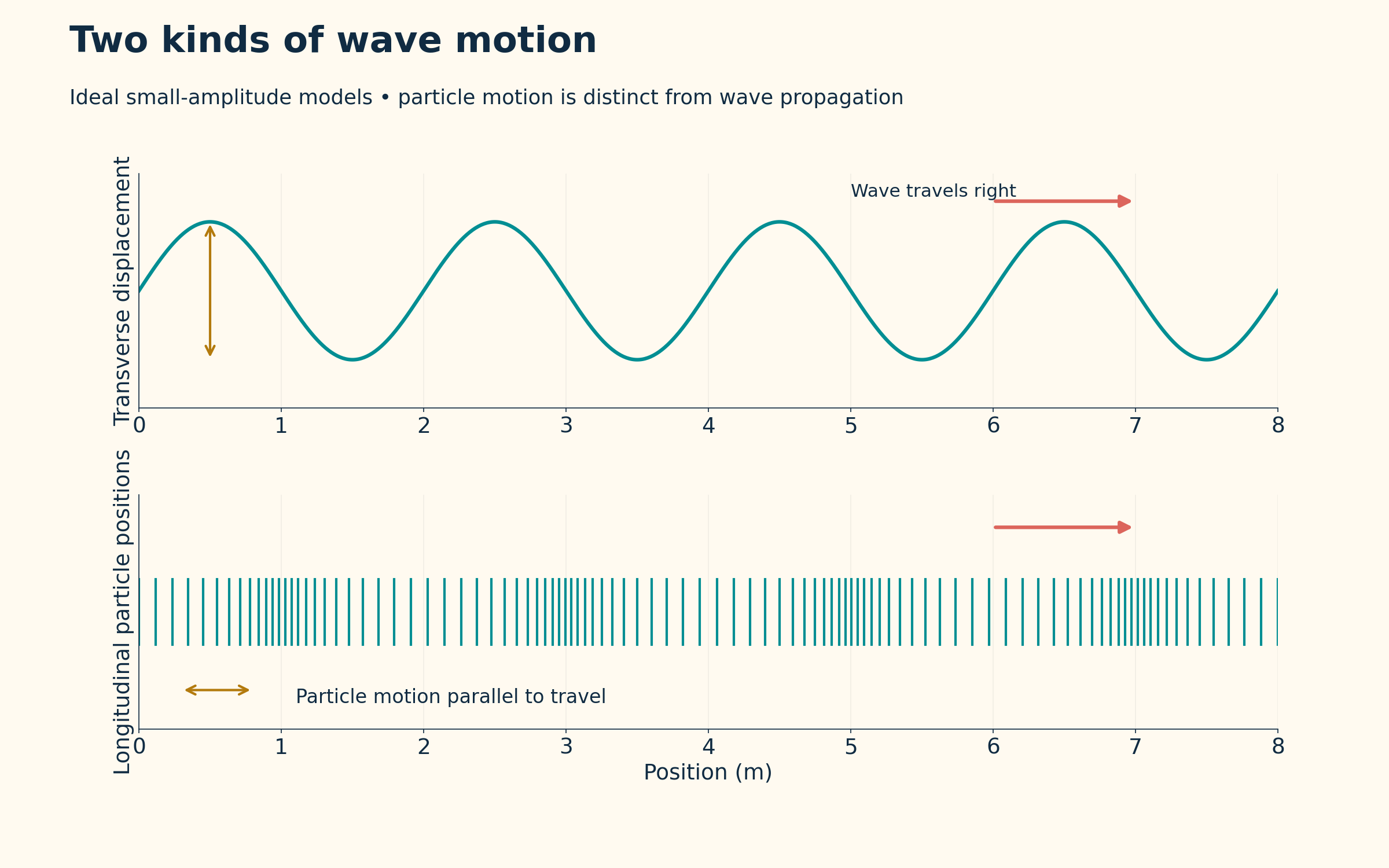

Wavelength and matching phase
A 2 m wavelength links equivalent phases in the wave representation.

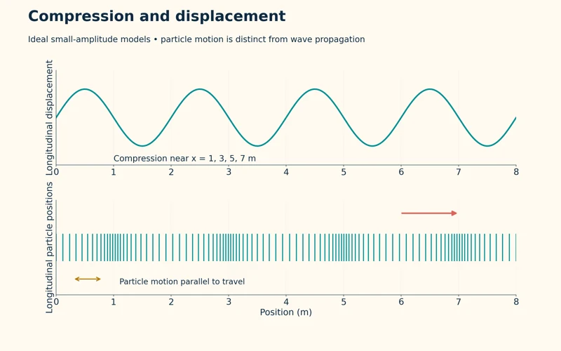
Compression and displacement
A displacement curve is paired with particle spacing to locate longitudinal compressions.
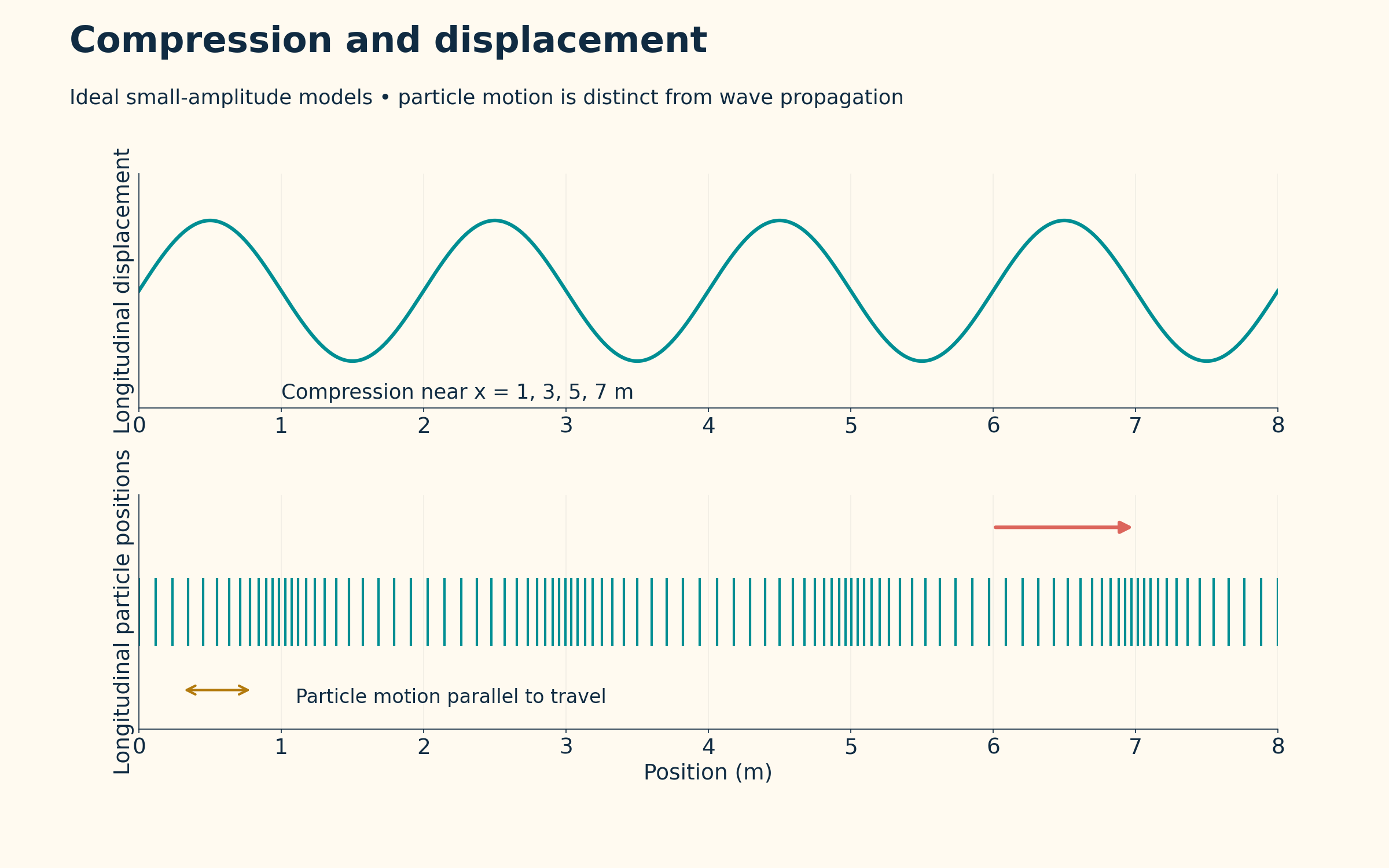
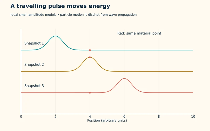
A travelling pulse
Three snapshots track a pulse moving right while one marked material point moves locally.


Reflection at a fixed end
A pulse approaching a fixed boundary returns inverted in an ideal reflected-wave model.

Ideal small-amplitude wave and pulse models. Particle motion is distinct from wave propagation; plotted snapshots and particle spacings are calculated representations.
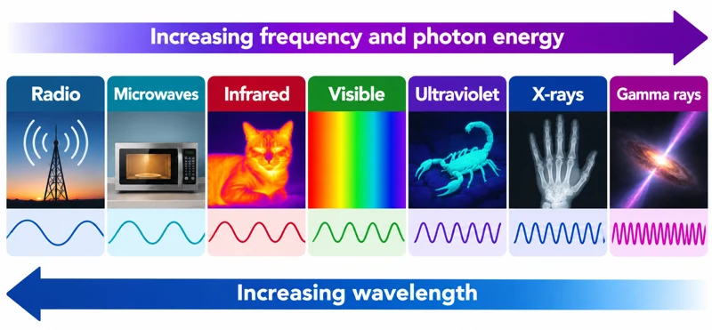 PHYSICS · 5 VISUALSElectromagnetic spectrumExplore electromagnetic regions, instruments and the relationships between wavelength, frequency and photon energy.
The spectrum in order
Radio through gamma-ray regions are arranged with increasing frequency and decreasing wavelength.
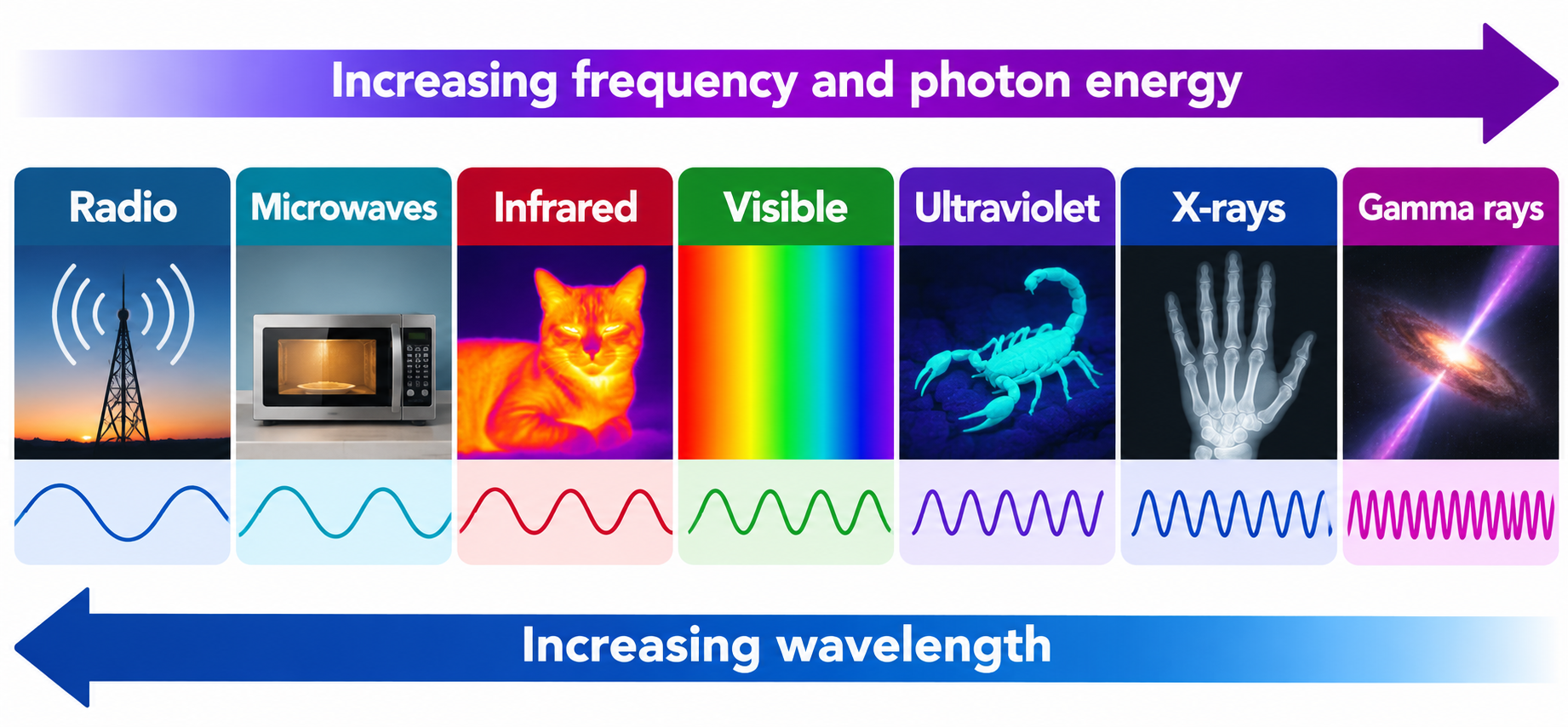

Familiar instruments
Examples connect spectrum regions with radio antennas, radar, thermal cameras, optical cameras and other detectors.


One electromagnetic family
The relation c = fλ links wavelength and frequency for electromagnetic waves in vacuum.


Photon energy across the spectrum
The relations E = hf = hc/λ connect increasing frequency with increasing photon energy.


A closer look at visible light
The full spectrum includes an enlarged red-to-violet band with approximate visible limits of 700 to 400 nm.

Illustrative spectrum overview, not a proportionally spaced wavelength scale. Region boundaries and visible limits are approximate; examples are not exclusive uses of each region.
 PHYSICS · 5 VISUALSRefraction and Snell lawUse the normal and refractive index to explain how a ray bends at a boundary.
Bending at a boundary
An air-to-glass ray bends towards the normal in an ideal refraction diagram.


Angles from the normal
A 45-degree incident ray enters glass at approximately 28.1 degrees to the normal.
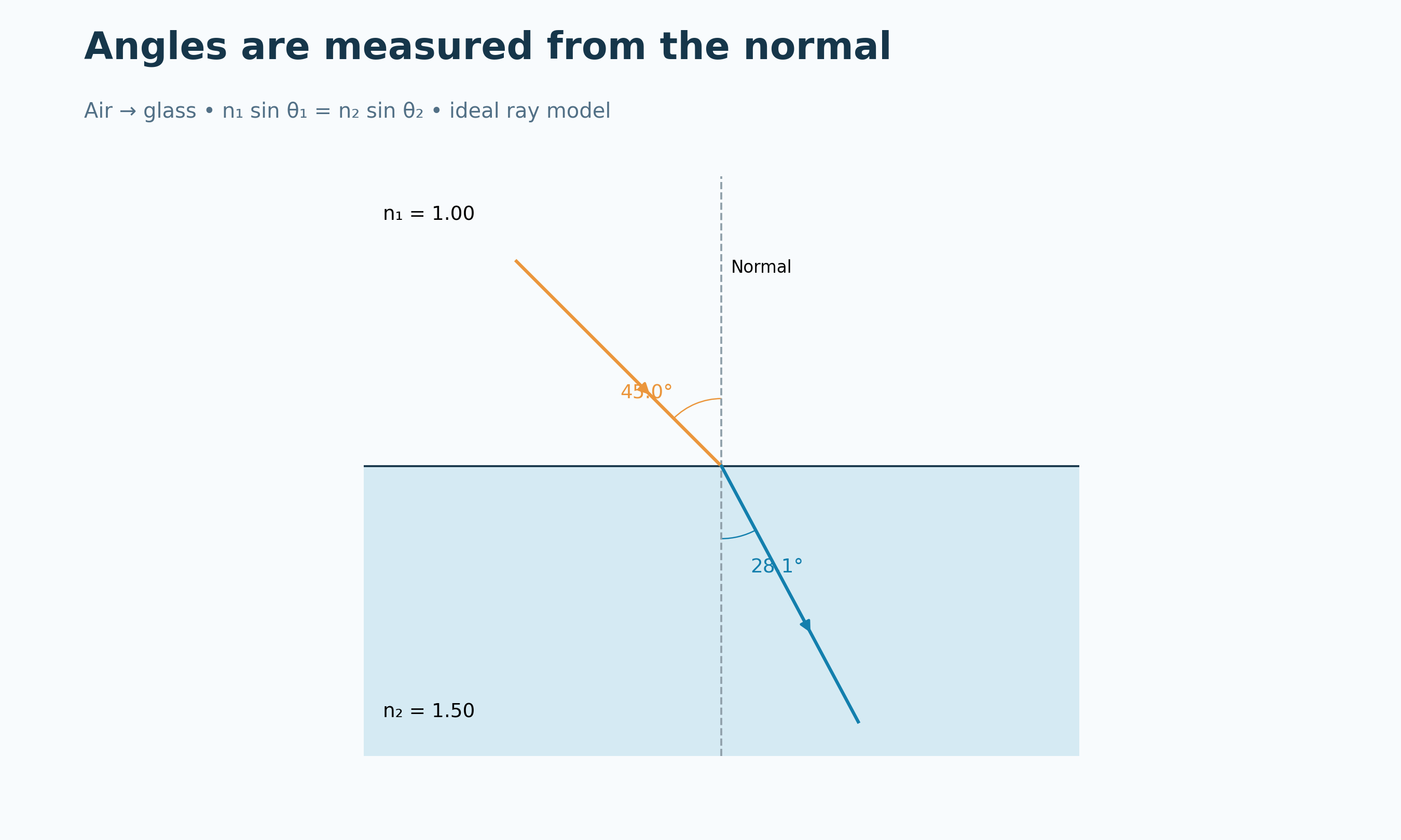

A numerical Snell example
Refractive indices 1.00 and 1.50 turn a 60-degree incident angle into approximately 35.3 degrees.
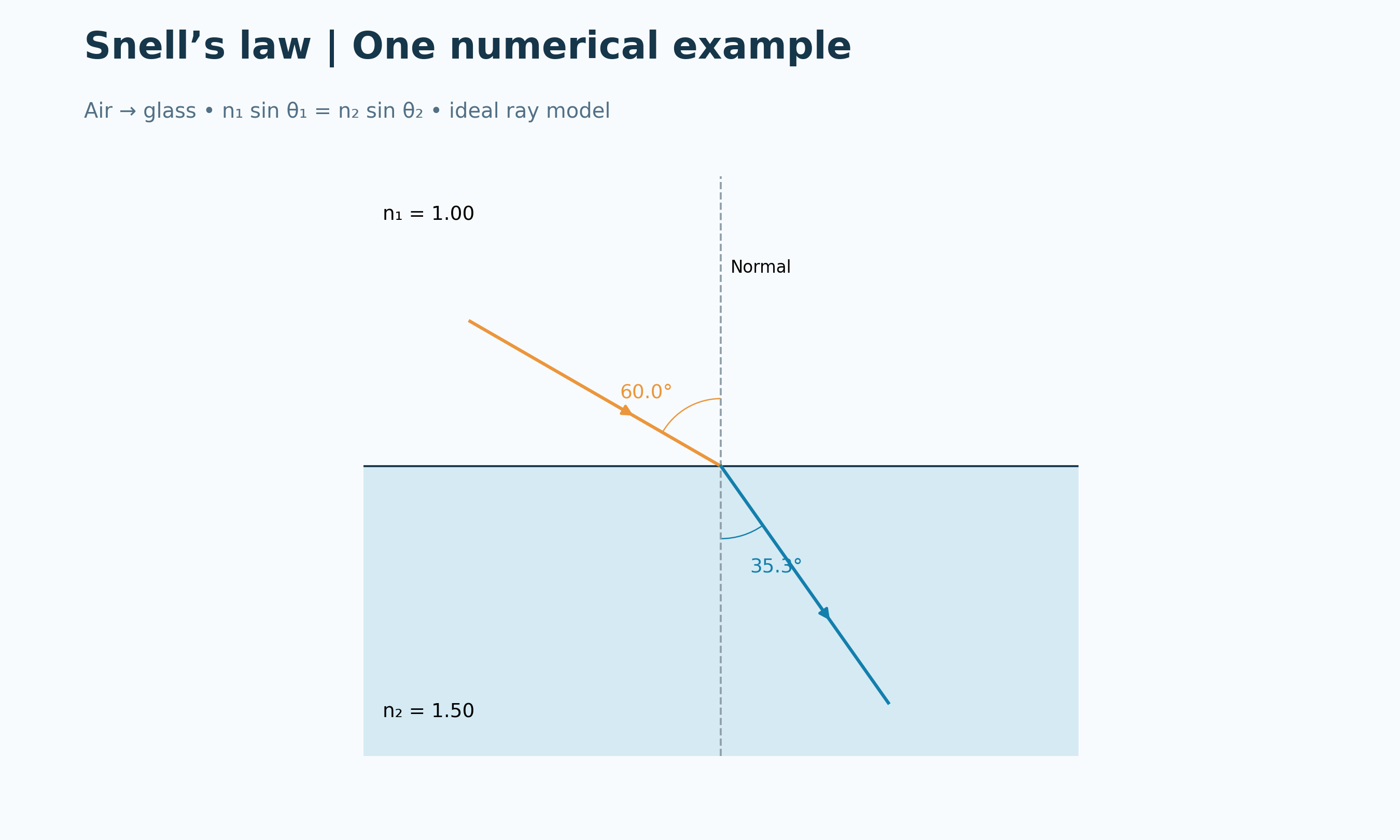

Reversing the path
A glass-to-air ray retraces the corresponding air-to-glass path.


A ray entering glass
An illustrative apparatus scene connects bending towards the normal with Snell’s law.

Ideal Snell-law geometry with angles measured from the normal. The apparatus image is qualitative and is not a calibrated optical photograph.
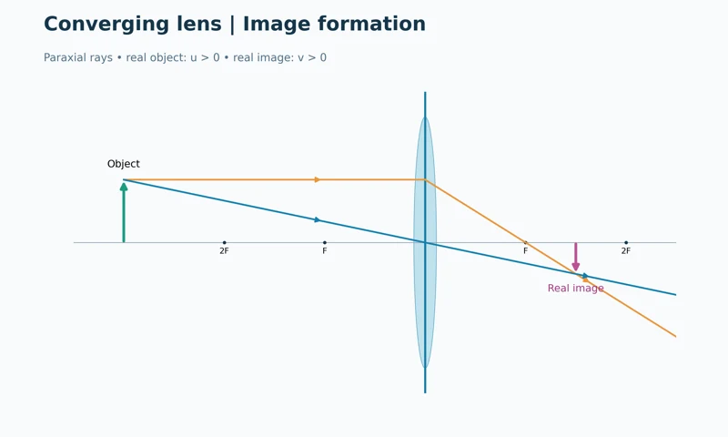 PHYSICS · 5 VISUALSConverging lens ray diagramConstruct real images with a converging lens and relate them to object distance.
Image formation
Two rays locate a reduced, inverted real image behind a converging lens.

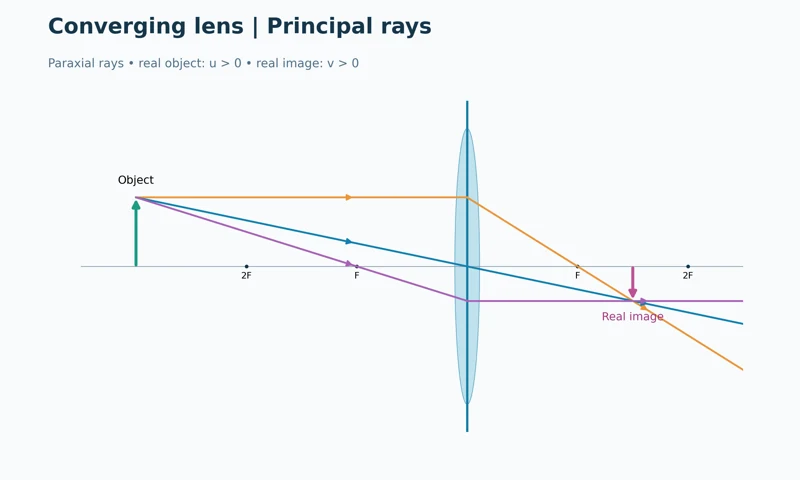
Three principal rays
Parallel, central and focal rays meet at the same image position.


Distances and magnification
An ideal f = 2 cm lens with u = 6 cm gives v = 3 cm and magnification −0.50.


A real image on a screen
An optical-bench illustration shows an inverted image formed on a screen for an object at three focal lengths.


Changing object distance
Three ray diagrams compare image distance and size for the same converging lens.
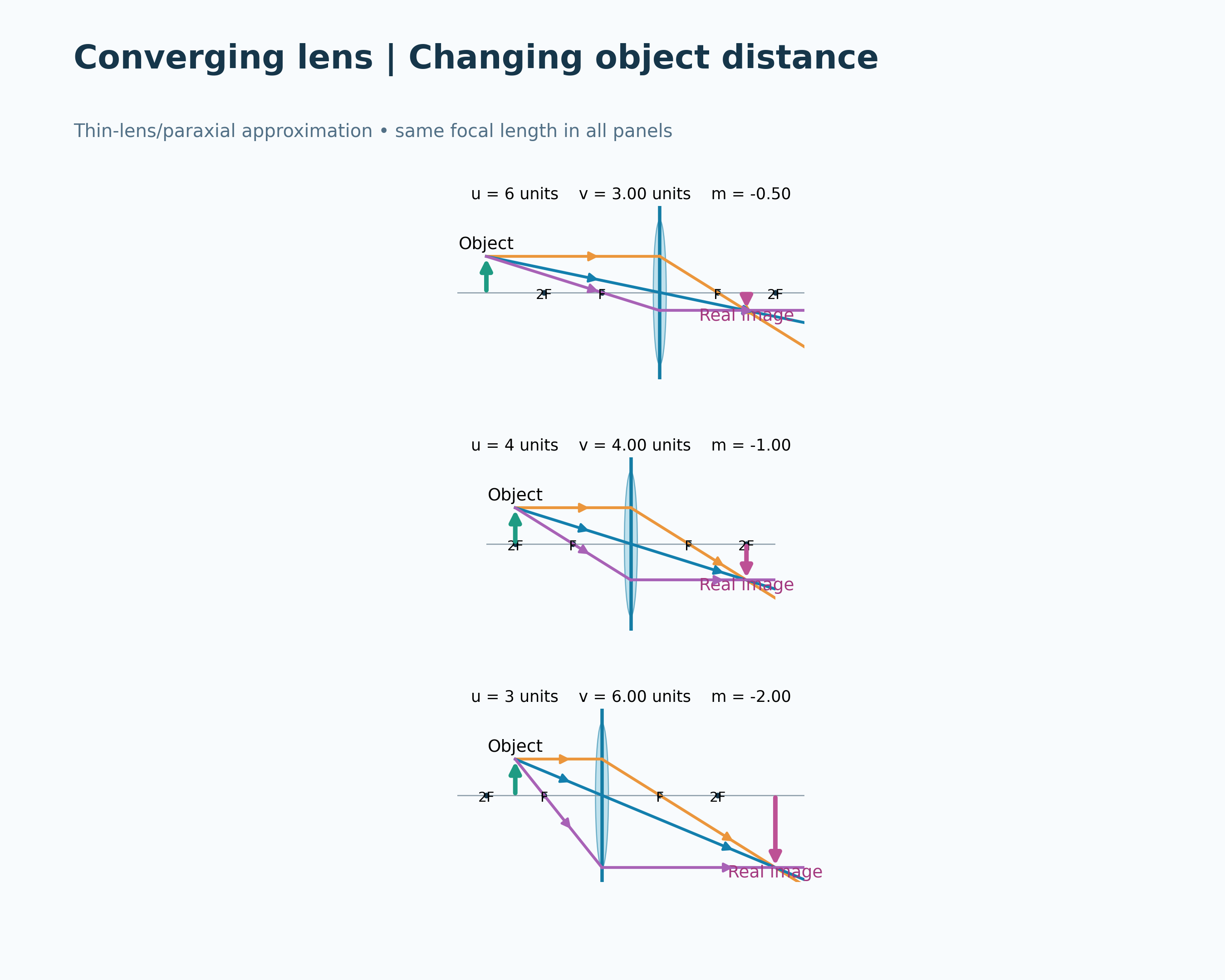
Thin-lens, paraxial ray model using the displayed distance convention. The optical-bench image illustrates the result but is not calibrated ray tracing or measured apparatus.
 PHYSICS · 5 VISUALSDiverging lens ray diagramLocate the upright virtual image produced by a diverging lens.
A reduced virtual image
Diverging rays and their backward extensions locate an upright image on the object side.
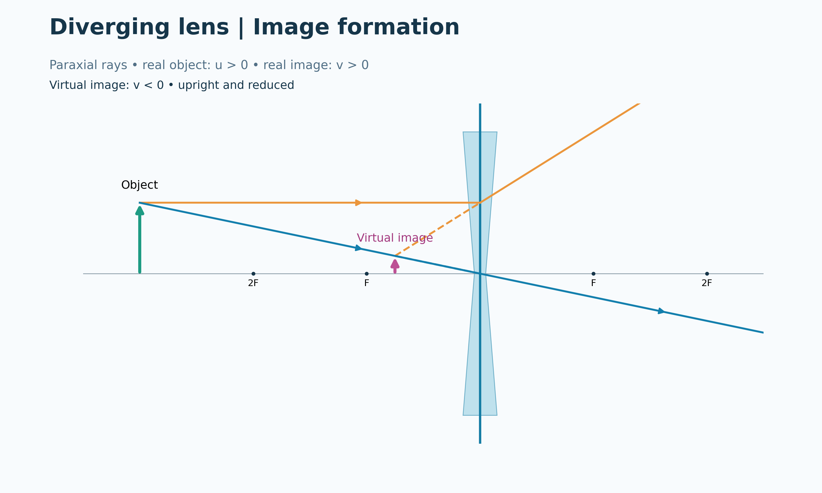
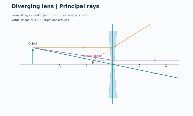
Principal rays
Three ray constructions locate the same virtual image between the lens and near focal point.
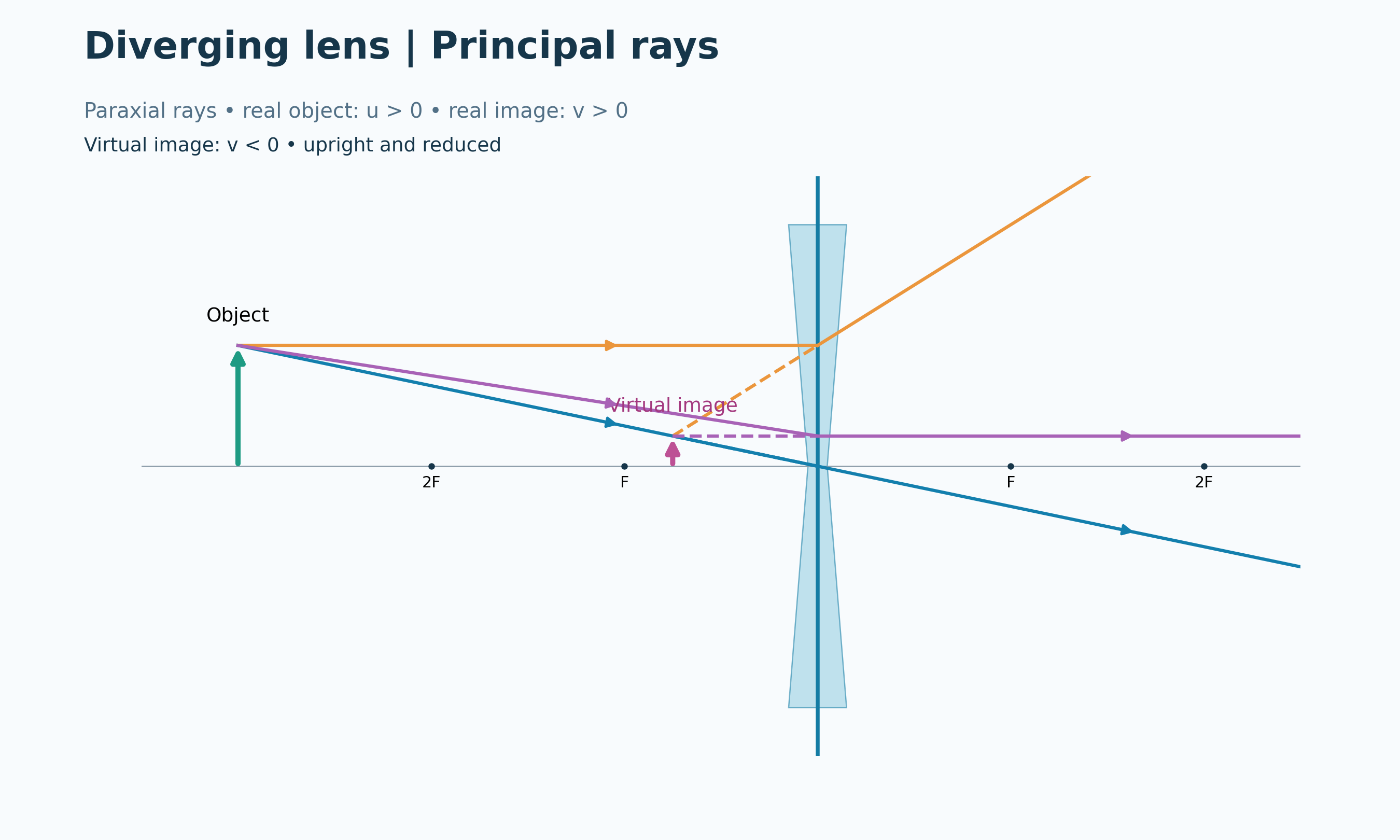

Signed distances
An ideal f = −2 cm lens with u = 6 cm gives v = −1.50 cm and magnification +0.25.


An upright, reduced view
A qualitative hand-held lens illustration shows smaller upright arrows through a diverging lens.


Correcting myopia
An idealised eye-lens model compares a focus before the retina with correction by a diverging lens.
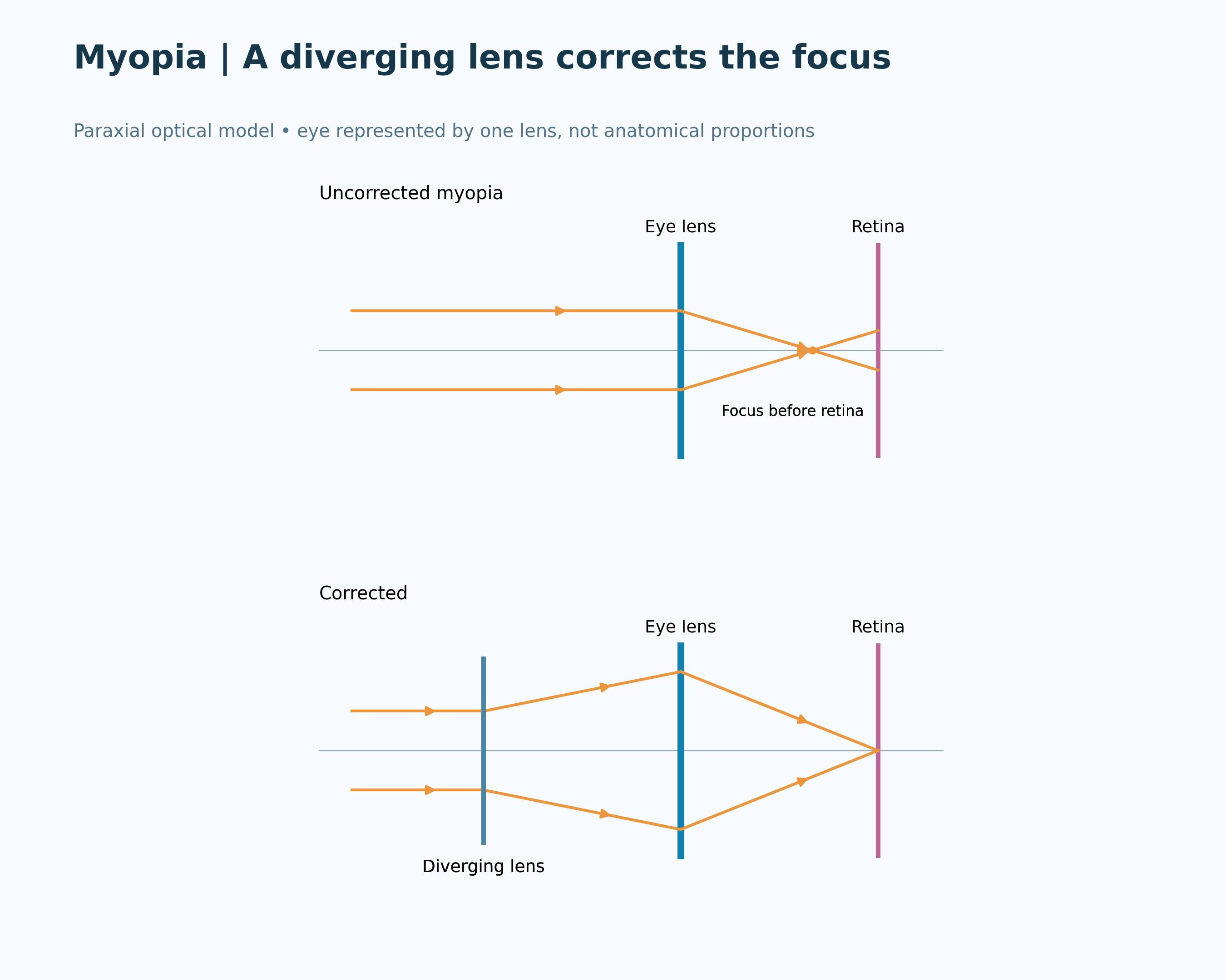
Thin-lens, paraxial model with negative focal length and negative virtual-image distance. The hand-held view is illustrative; the myopia diagram is an optical model, not an anatomical drawing.
 PHYSICS · 5 VISUALSElectric dipole field linesConnect electric dipole field direction, equipotentials and force on a test charge.
Opposite charges
Field lines show the pattern around equal positive and negative point charges.

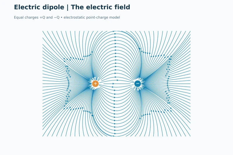
The dipole field
A denser field-line view displays the electrostatic pattern of an equal-charge dipole.
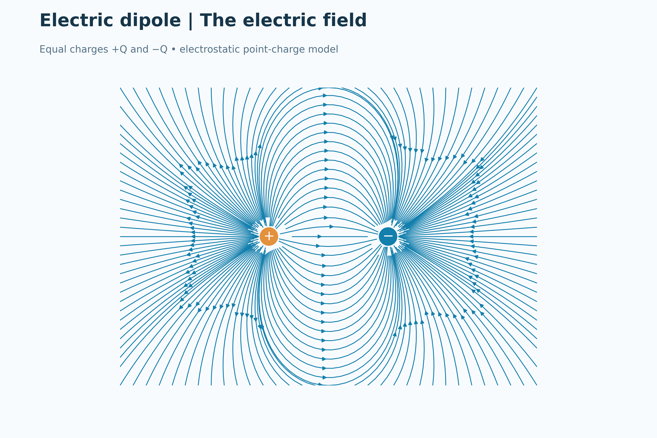

Equipotential curves
Positive and negative potential contours surround the charges, with zero potential on the central perpendicular line.


Field and potential together
Overlaid field lines and potential contours show their perpendicular relationship.


A positive test charge
Force arrows on positive test charges point along the local electric field.

Calculated electrostatic point-charge field and potential for equal opposite charges. Singular regions are masked and the finite frame crops field lines; test-charge arrows indicate direction qualitatively.
 PHYSICS · 5 VISUALSBar-magnet field/iron filingsRead magnetic field direction and distinguish field-line models from iron-filings patterns.
Field around a bar magnet
A schematic bar magnet has field arrows from north to south outside the magnet.
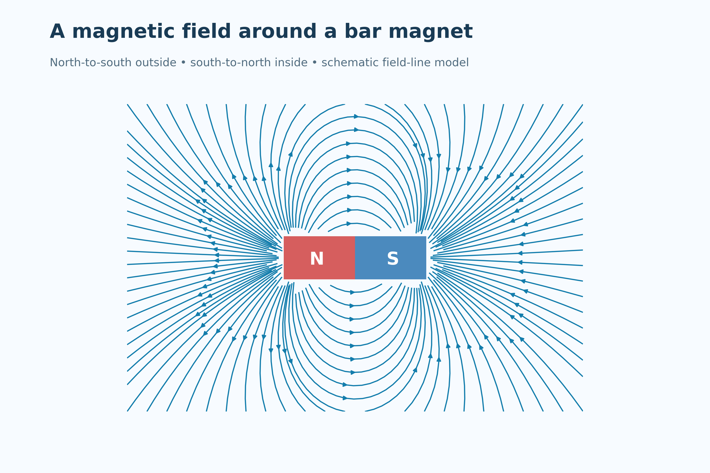

Compass directions
Compass needle tips align with the local magnetic field at several positions.
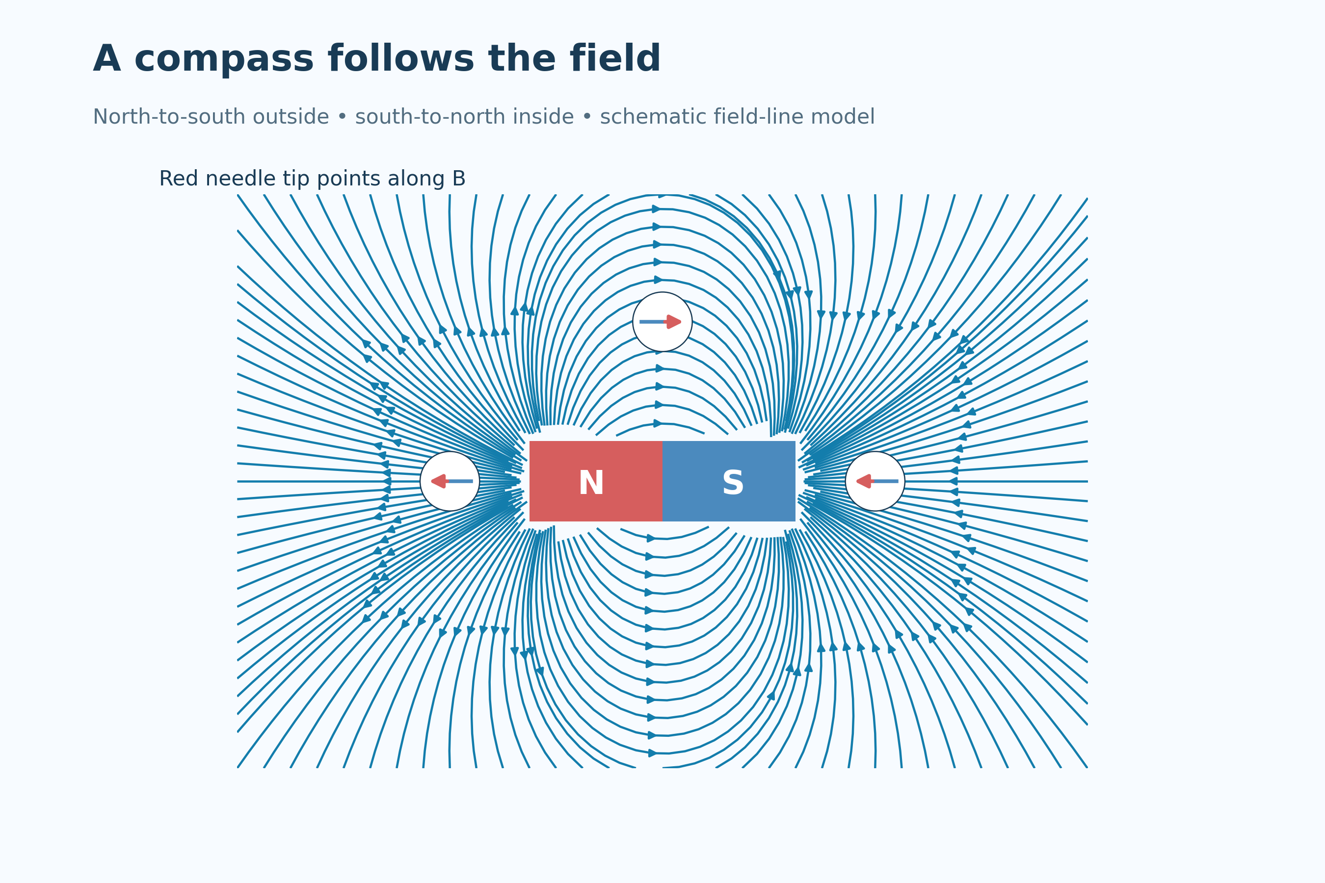

Closed field loops
Interior arrows run south to north, completing the conceptual magnetic field loops.


Field strength near the poles
More closely spaced lines illustrate the stronger field near the poles.
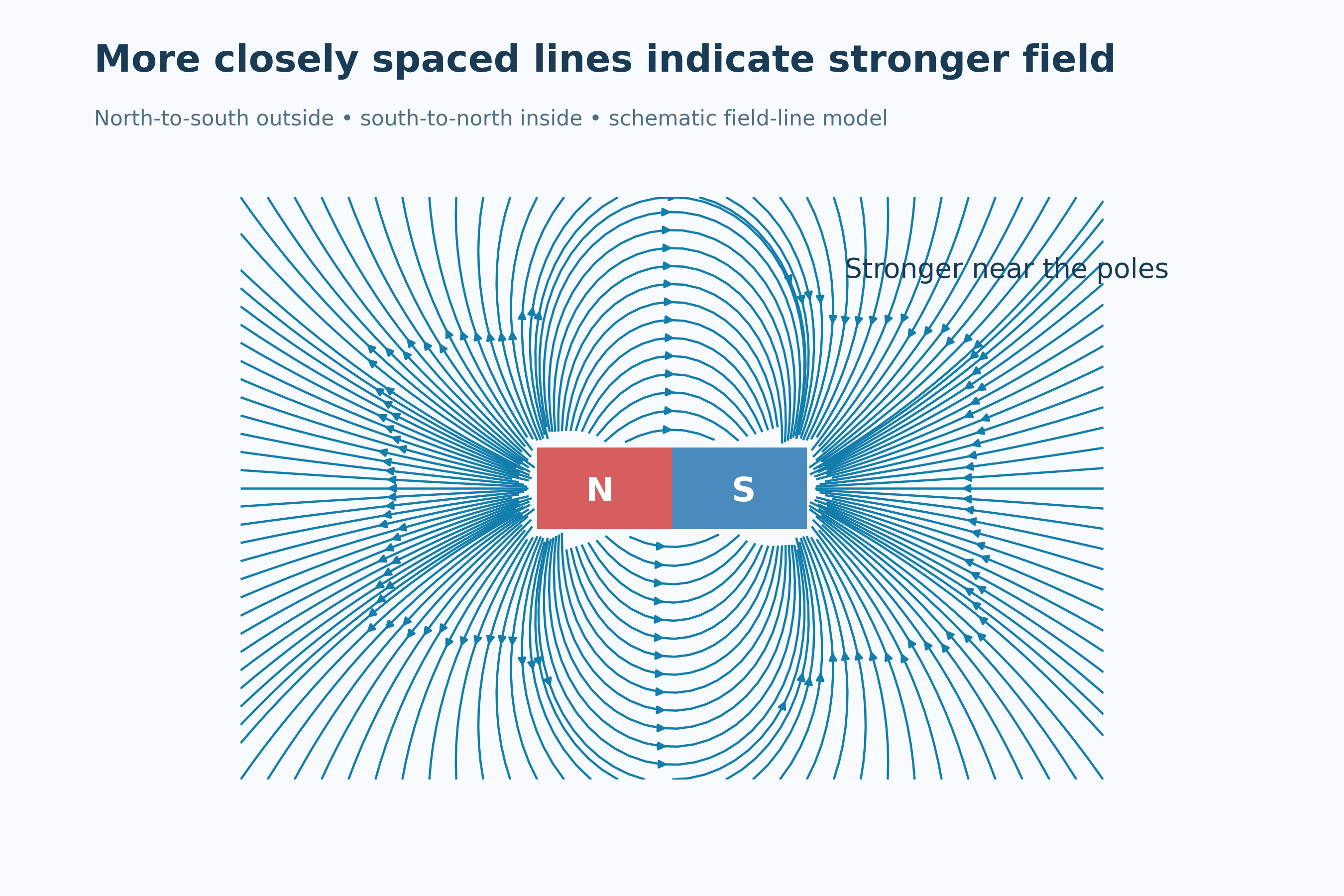

Iron-filings pattern
An illustrative filings arrangement reveals the field pattern without independently indicating direction.
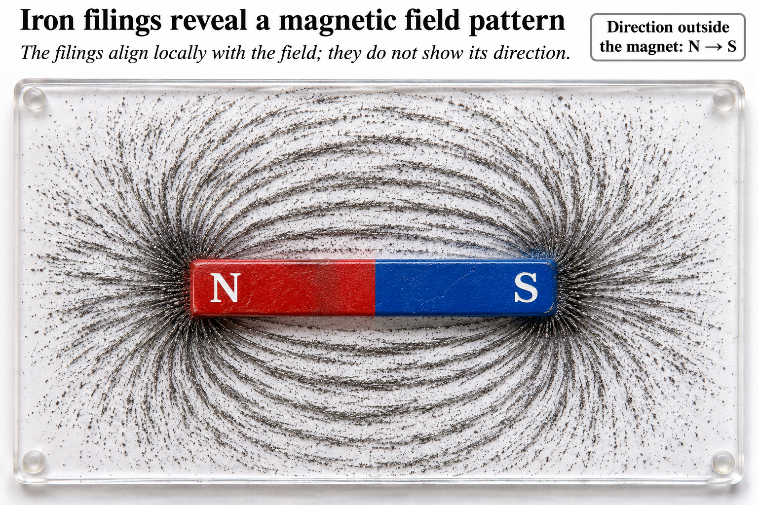
Qualitative bar-magnet field model. An exterior equivalent-pole construction and interior arrows illustrate direction and closed loops, not literal magnetic charges. The filings scene is illustrative.
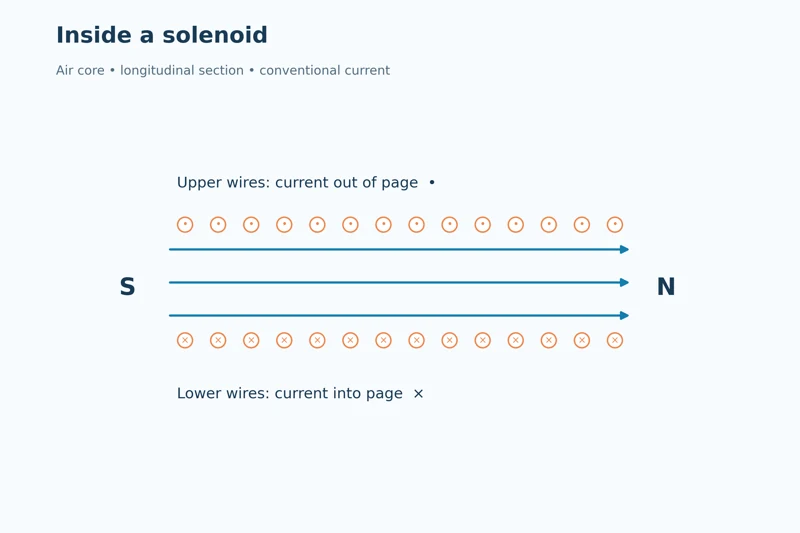 PHYSICS · 5 VISUALSSolenoid magnetic fieldConnect solenoid current direction, magnetic poles and the long-solenoid approximation.
Inside a solenoid
A longitudinal section uses dots and crosses for current and arrows for the internal field.
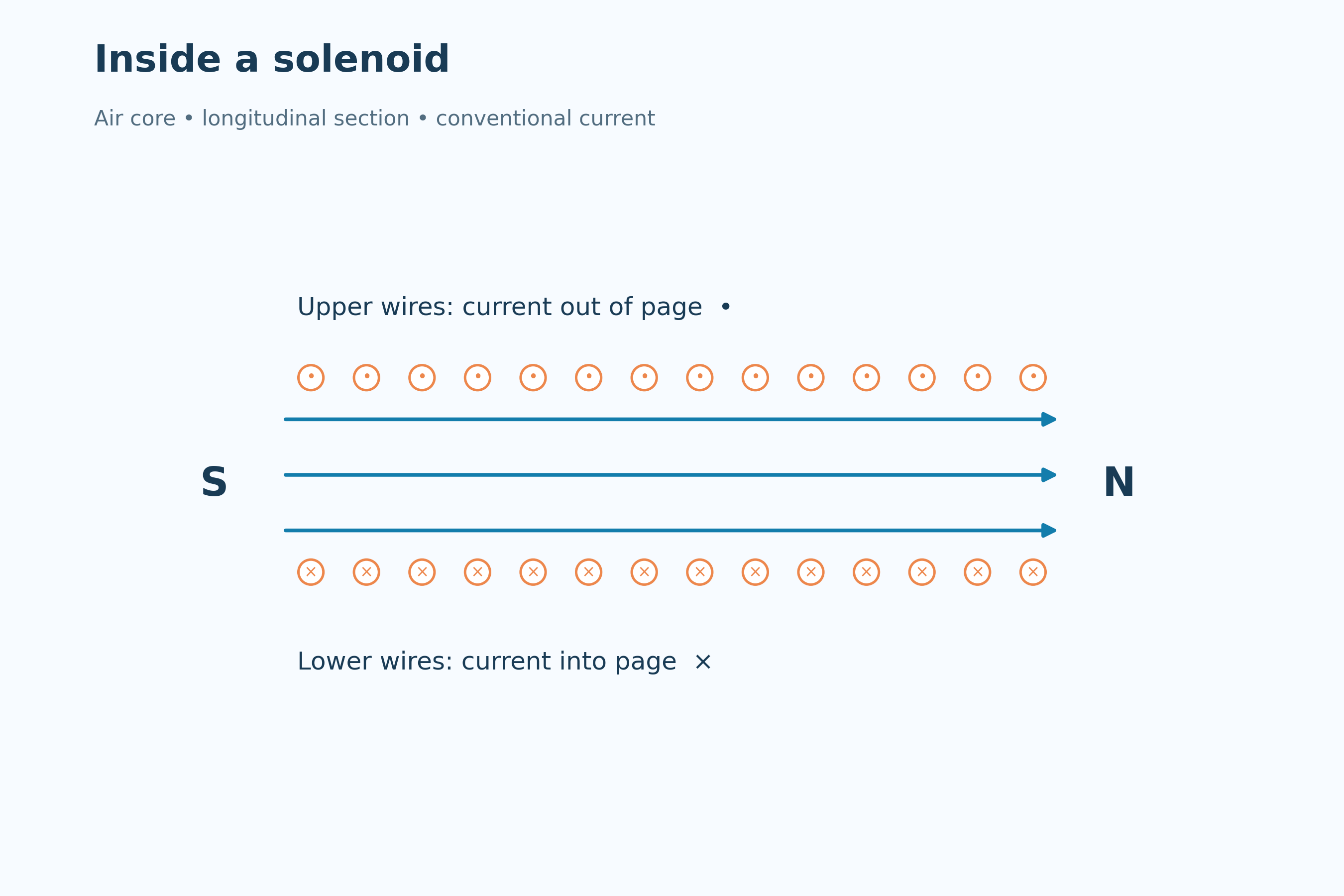

Current fixes the poles
The north-end view links counterclockwise conventional current with the north pole.
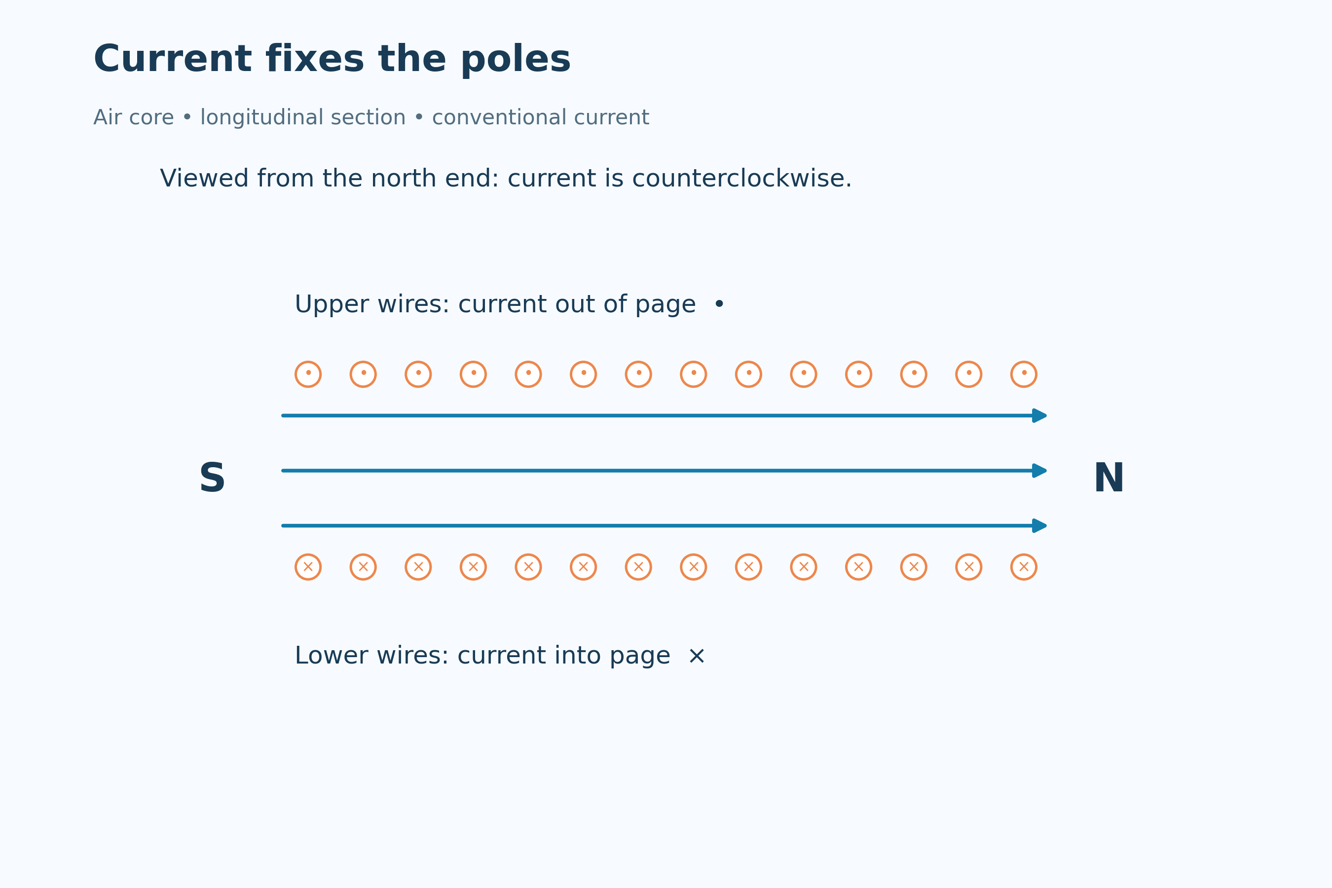
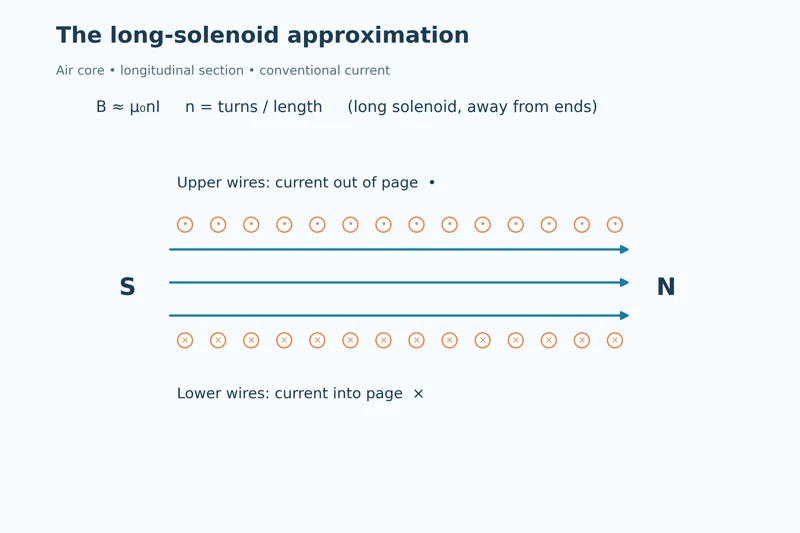
The long-solenoid approximation
B ≈ μ₀nI relates field strength to current and turns per length in an air-core model.


Doubling the current
At unchanged turns per length, doubling current doubles the ideal internal field.


A long air-core coil
A detailed coil illustration connects winding direction, poles and the approximately uniform internal field.

Ideal long air-core solenoid, away from its ends. The longitudinal cross-sections use conventional current; the detailed coil is a qualitative illustration.
 PHYSICS · 5 VISUALSElectromagnetic inductionRelate changing magnetic flux to induced emf and Lenz’s law.
An approaching magnet
An illustrative coil and meter show induction as a north pole approaches, with current viewed from the magnet.


Approaching and withdrawing
End-on coil diagrams compare opposite induced current directions for approach and withdrawal.


The minus sign in Faraday’s law
An increasing positive flux curve is paired with its negative induced-emf curve.


Faster change, larger peak emf
Two equal flux changes over different time intervals compare their induced-emf peaks.


Flux differs from emf
Linked graphs show emf approaching zero as flux becomes nearly constant.

Ideal changing-flux examples with a chosen coil orientation. Emf curves follow the negative flux derivative; they do not determine current magnitude without circuit impedance. The apparatus is illustrative.
 PHYSICS · 5 VISUALSCircular motion: velocity and accelerationSeparate tangential velocity from inward acceleration in uniform circular motion.
Turning without slowing
A particle has tangential velocity and inward acceleration while its speed remains constant.


Velocity around the circle
Four positions show perpendicular tangential velocity and radial acceleration.
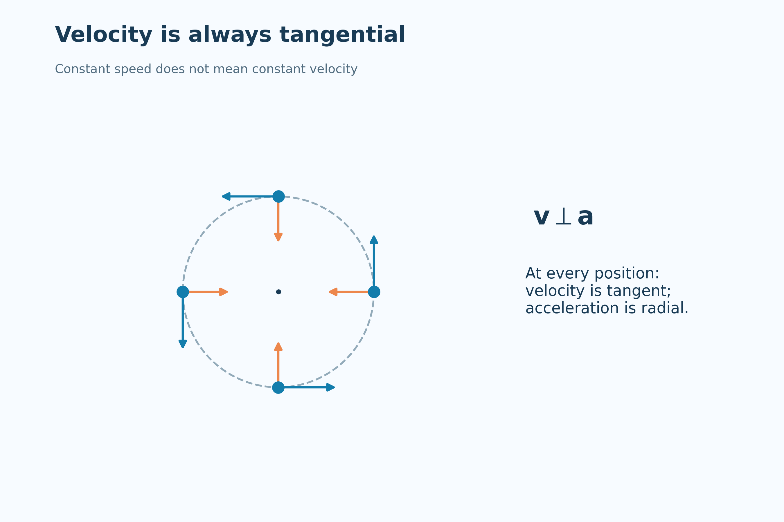

Changing velocity direction
The relation a = v²/r connects inward acceleration with speed and radius.


Doubling speed
At radius 2.0 m, increasing speed from 2.0 to 4.0 m/s increases acceleration from 2.0 to 8.0 m/s².


Tension supplies the inward force
A puck on a smooth horizontal table illustrates tension providing the net centripetal force.

Uniform circular-motion model. Arrows show directions rather than a common comparative magnitude scale. The puck scene is a qualitative top view with weight and normal force balanced.
 PHYSICS · 5 VISUALSHalf-life curveRead exponential decay, half-life and activity without confusing expected populations with individual random events.
An exponential decay curve
The expected number of undecayed parent nuclei decreases according to the half-life relation.


Successive halves
Equal time intervals reduce an initial 800 nuclei to 400, 200, 100 and 50.


Activity follows the same law
Activity values in becquerels halve over successive half-lives, separately from the nucleus count.


Random events and predictable populations
A simulated sample is compared with the expected decay curve and a logarithmic transformation.


An eight-hour half-life
An initial activity of 800 Bq falls to 100 Bq after 24 hours in the worked example.

Exponential expected population and activity models, plus one simulated random sample of independent decays. The numerical half-life is 8 hours; plotted curves are not measured radioactive samples.
 PHYSICS · 5 VISUALSSpring extension and Hooke lawMeasure extension from natural length and distinguish Hooke’s law from elastic behaviour.
Length and extension
An unloaded and loaded spring distinguish natural length L₀ from extension x.
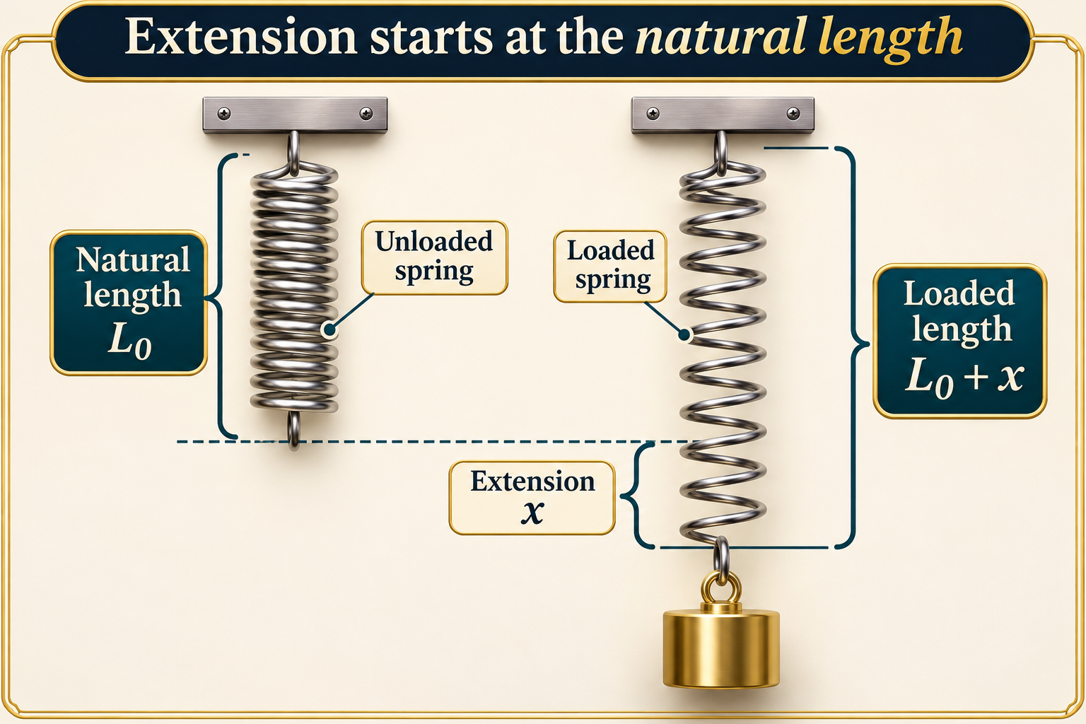

Force proportional to extension
Identical springs show force F giving extension x and force 2F giving extension 2x within the proportional range.


Calibrating a spring
A labelled setup measures unloaded and loaded pointer readings against a fixed ruler.

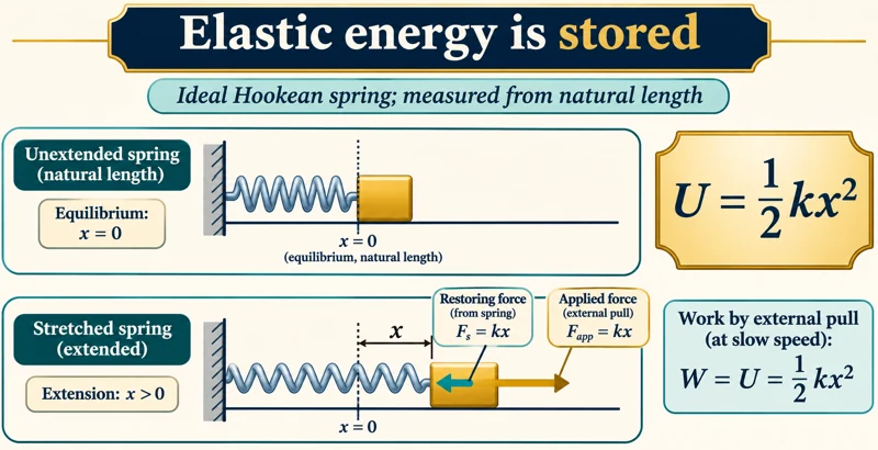
Elastic energy storage
A slowly stretched ideal spring links restoring force, external work and U = ½kx².


Proportional is not the same as elastic
Comparisons distinguish a straight-line force-extension relation, elastic recovery and permanent deformation.
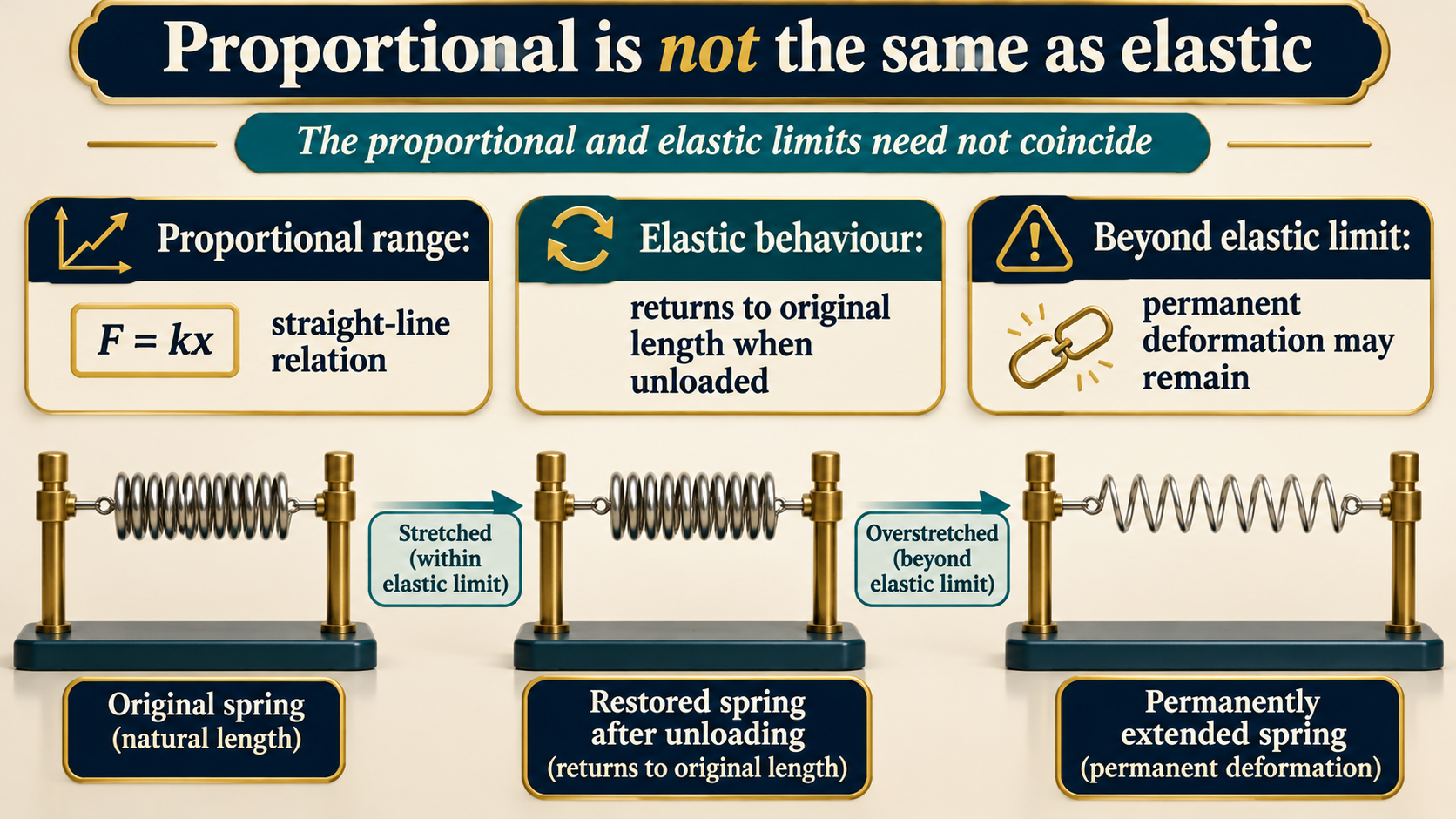
Ideal Hookean relationships apply within the proportional range. Apparatus and deformation comparisons are illustrative, not measured spring data. Proportional and elastic limits need not coincide.
 PHYSICS · 5 VISUALSSHM displacement and periodConnect an oscillating spring’s positions with displacement, period and frequency.
Three oscillator positions
A spring at +A, zero and −A is paired with a displacement graph.


Five phases of one cycle
Spring snapshots at quarter-period intervals match a cosine displacement curve.


A cosine displacement model
A = 0.10 m and angular frequency π rad/s define the plotted displacement.


Period and frequency
A two-second period corresponds to a frequency of 0.50 Hz.


Matching position and motion
Quarter-cycle spring positions include velocity-direction arrows alongside the displacement graph.

Ideal undamped horizontal-spring oscillator starting at its right-hand extreme. Displacement is measured from equilibrium; the equation example has amplitude 0.10 m and period 2.0 s.
 PHYSICS · 5 VISUALSSHM displacement/velocity/acceleration phasesRelate SHM displacement, velocity and acceleration through phase and derivatives.
Three linked quantities
Aligned displacement, velocity and acceleration graphs show a two-second oscillation.


Zeros and extrema
Quarter-cycle markers compare zero crossings with maximum and minimum values.


Derivatives determine the signs
The graphs connect v = dx/dt, a = dv/dt and a = −ω²x.


A complete cycle
Marked phases track the same oscillator through one full period.

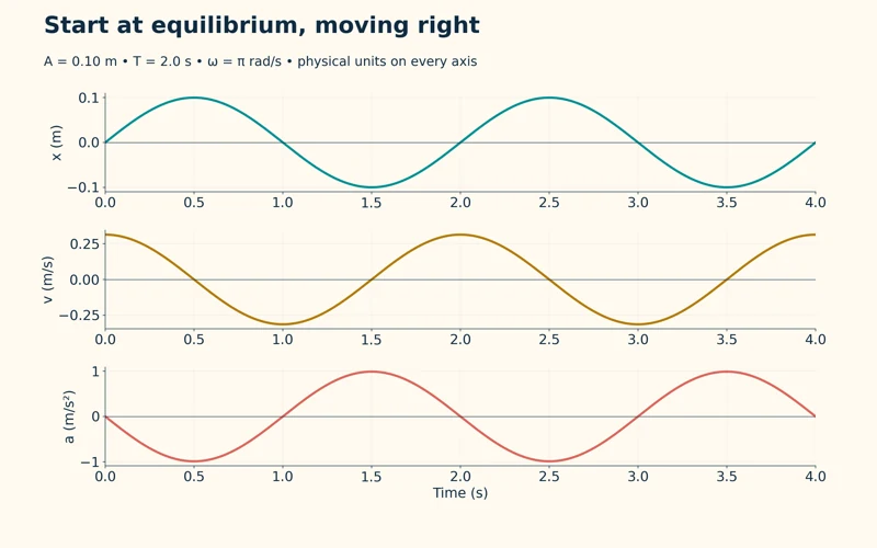
Starting from equilibrium
A different initial phase starts at zero displacement while moving right.

Calculated ideal SHM curves with amplitude 0.10 m, period 2.0 s and angular frequency π rad/s. The final view changes the initial phase, not the underlying SHM relations.
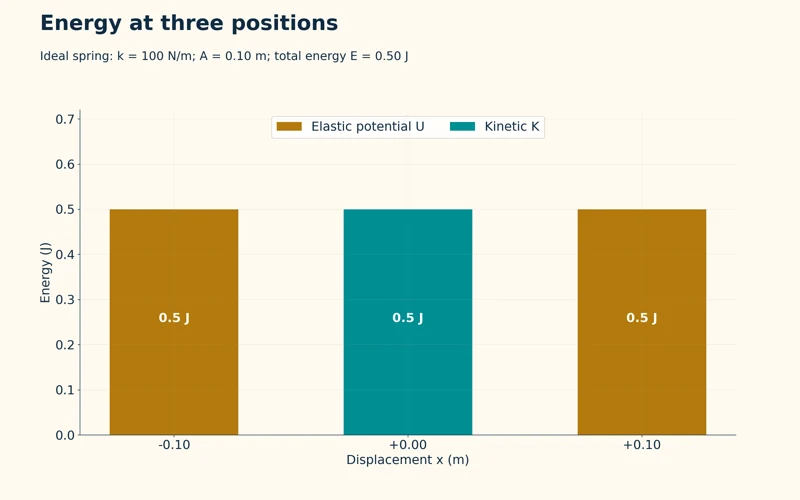 PHYSICS · 5 VISUALSSHM kinetic/potential energyTrack kinetic and elastic potential energy during simple harmonic motion and damping.
Energy at three positions
Energy bars show all elastic potential energy at the extremes and all kinetic energy at equilibrium.
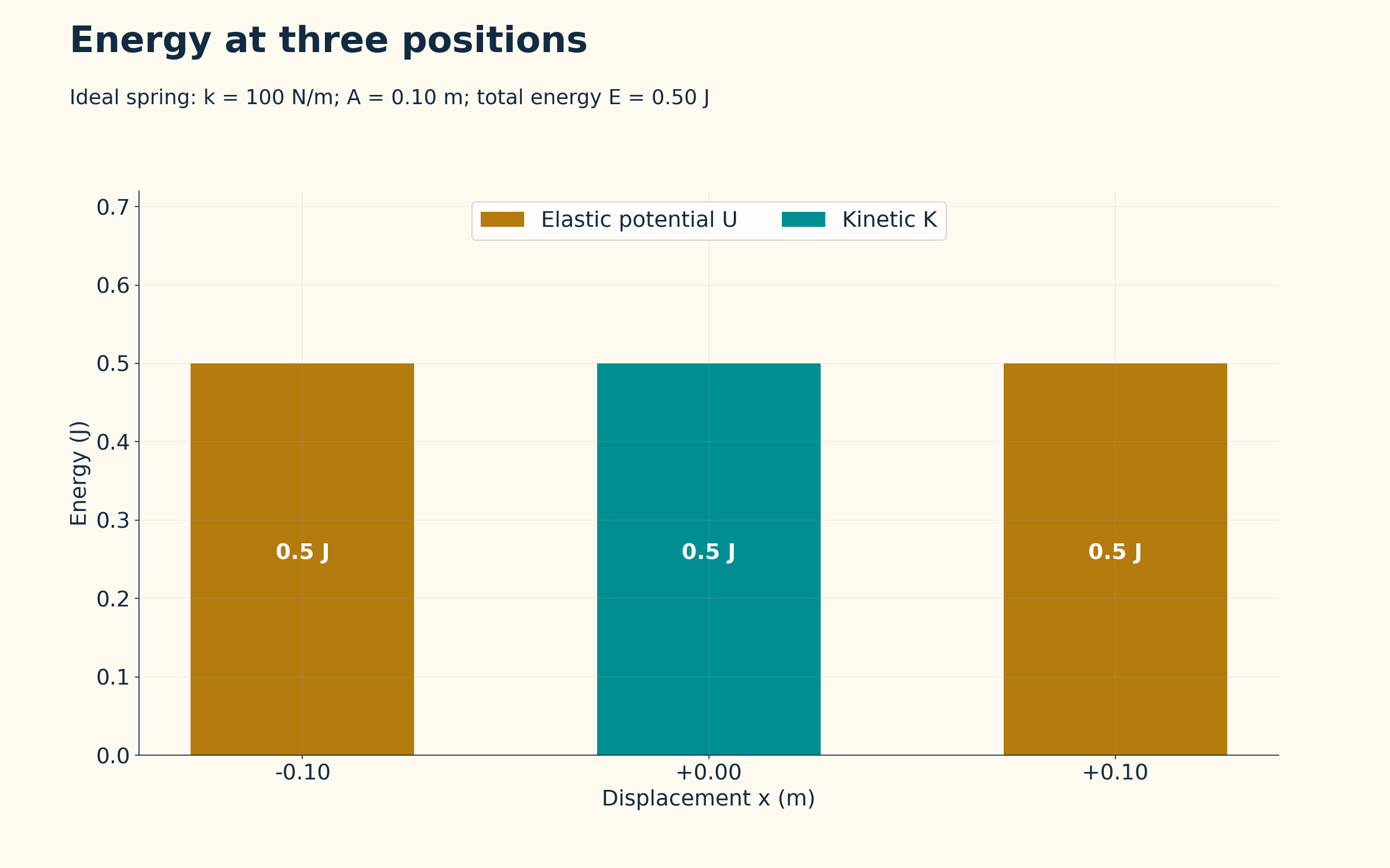

Equal totals throughout
Five displacement positions share a total mechanical energy of 0.50 J in the ideal spring model.
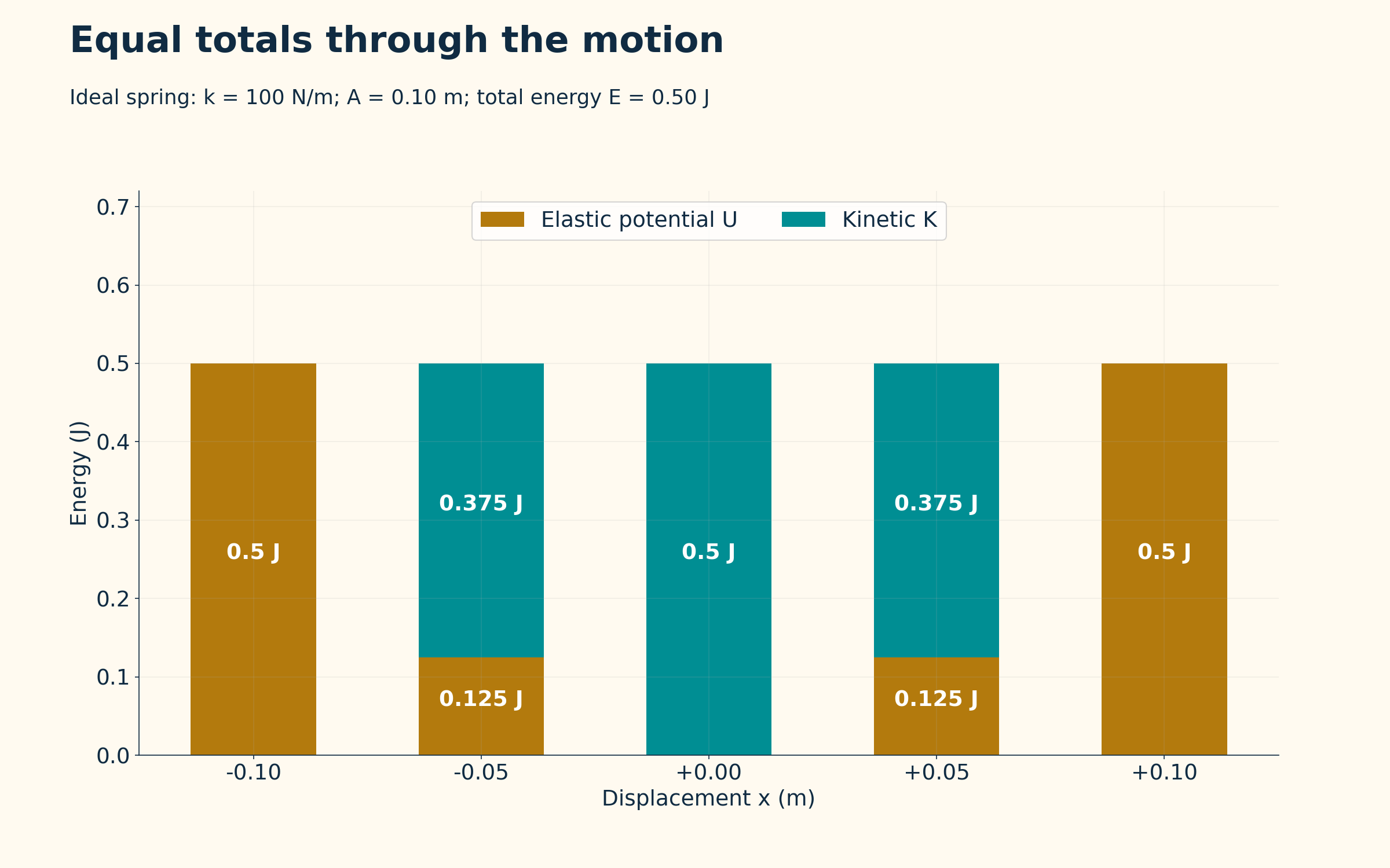

Energy versus displacement
Parabolic potential and kinetic-energy curves add to the constant total.
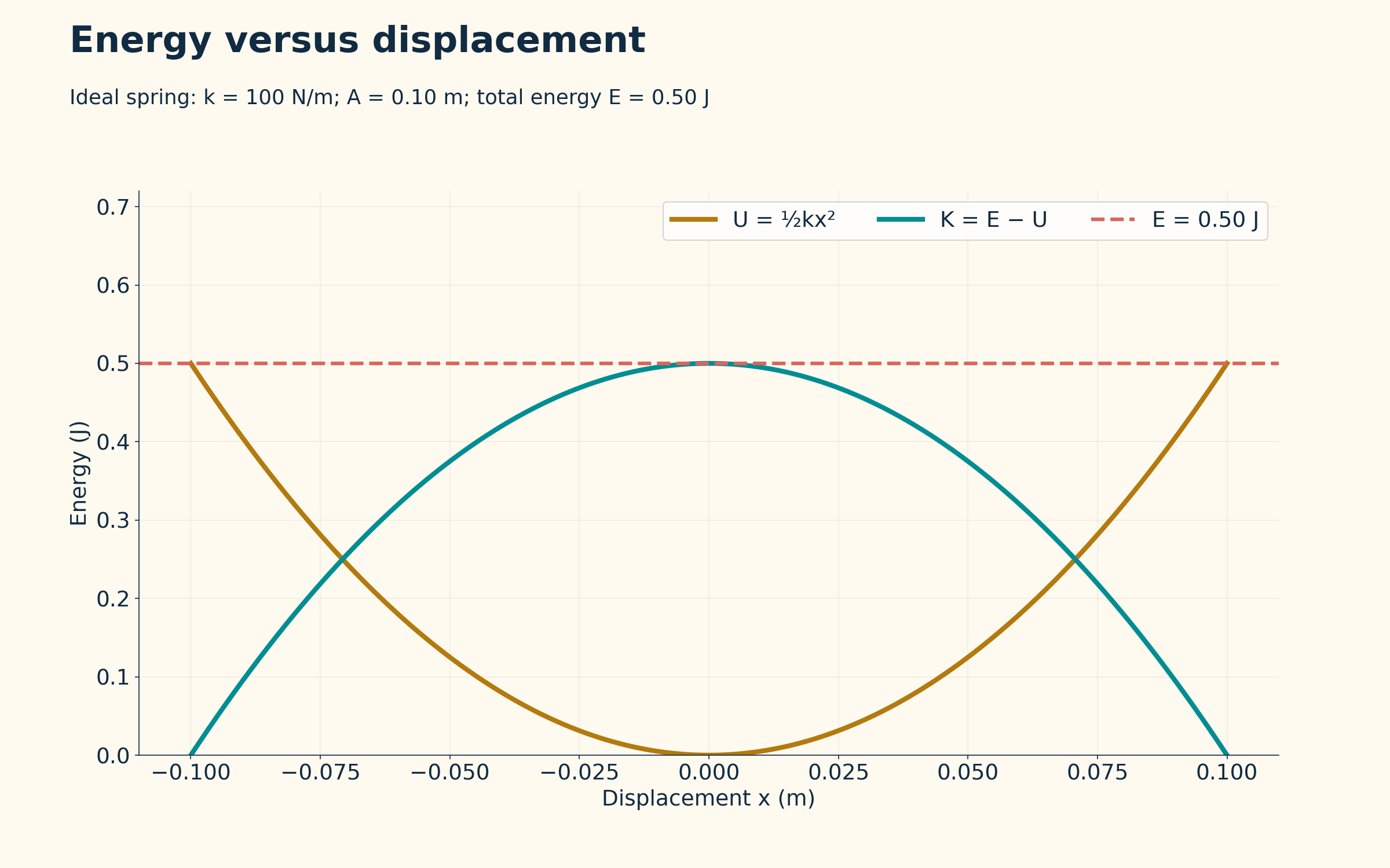
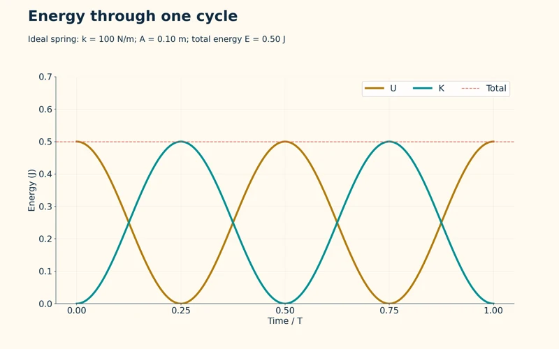
Energy through one cycle
Kinetic and potential energies exchange while their sum stays at 0.50 J.


Damping transfers energy
A cycle-averaged model shows mechanical energy decreasing as the thermal energy of oscillator and surroundings increases.

Ideal spring model with k = 100 N/m, amplitude 0.10 m and total mechanical energy 0.50 J. The damping view is a cycle-averaged illustration for oscillator plus surroundings, not measured data.
 PHYSICS · 5 VISUALSStanding waves, nodes and antinodesLocate standing-wave nodes and antinodes and connect harmonics with wavelength and frequency.
The fundamental mode
A string fixed at both ends has end nodes and one central antinode.

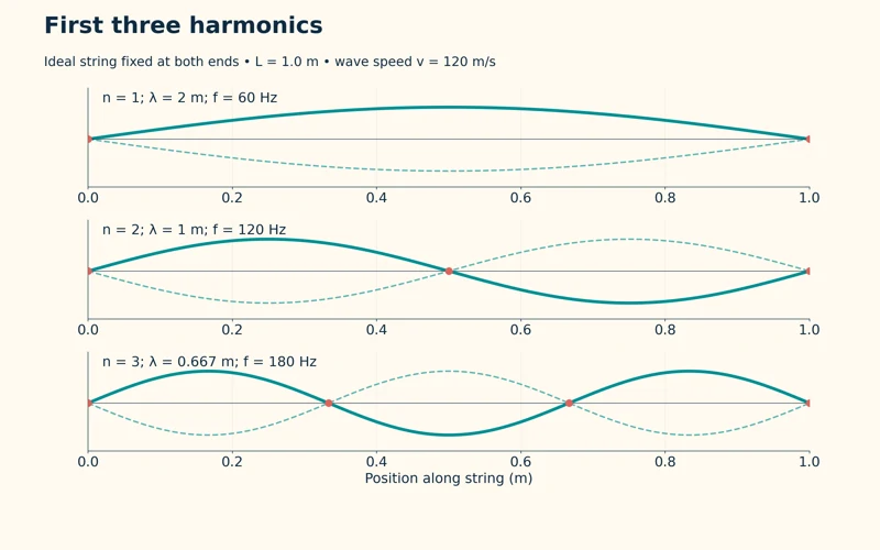
First three harmonics
Three modes on a 1.0 m string have frequencies of 60, 120 and 180 Hz for wave speed 120 m/s.


Counting nodes
Comparisons mark zero, one and two internal nodes for the first three harmonics.
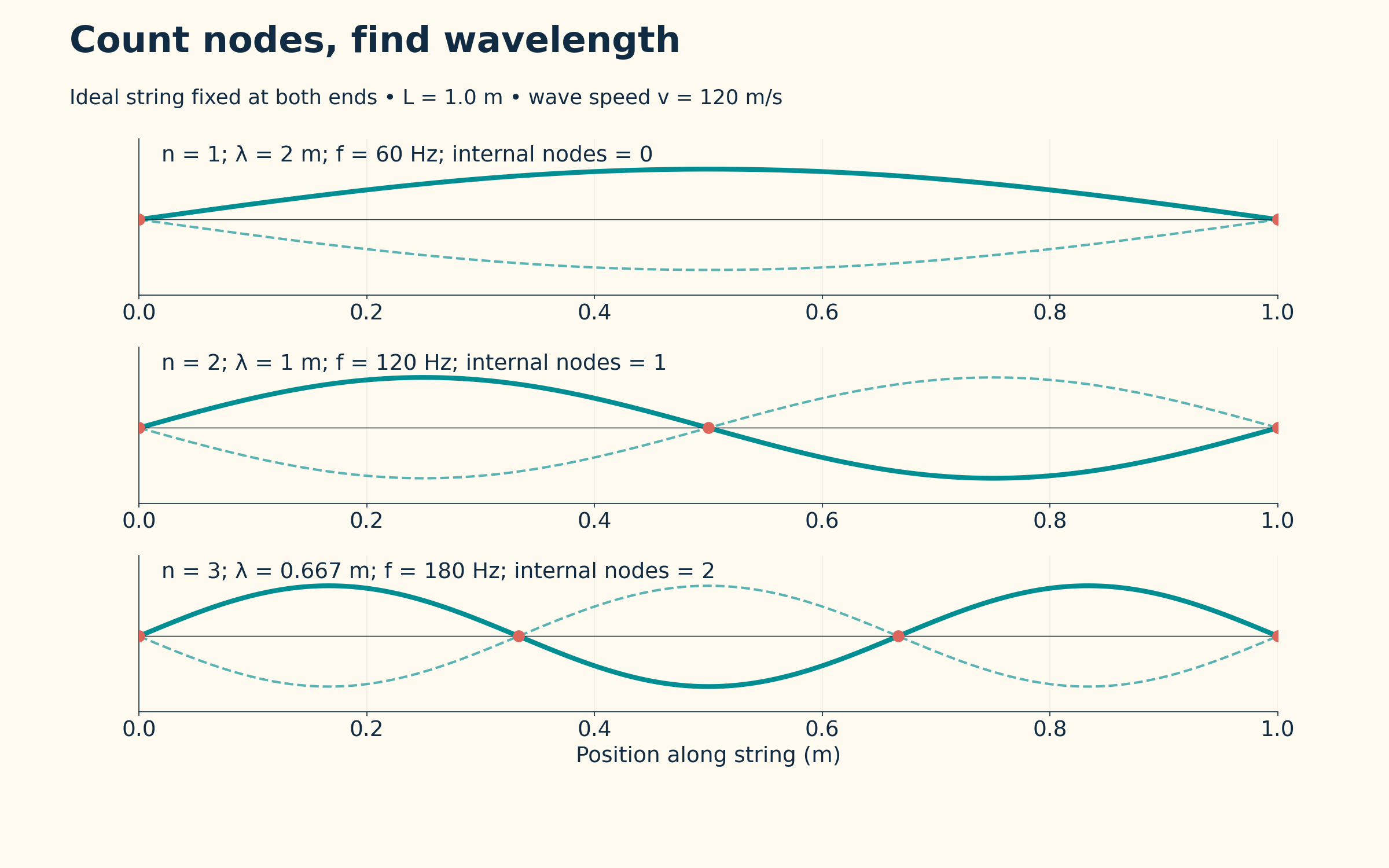
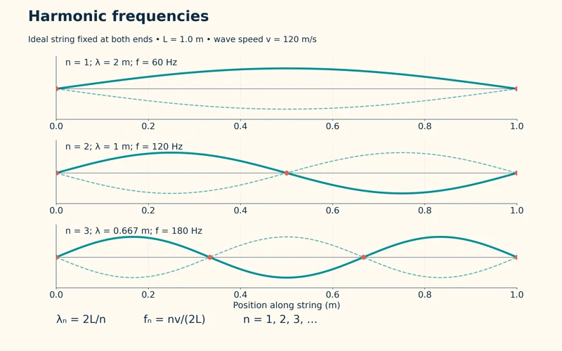
Harmonic frequencies
The relations λₙ = 2L/n and fₙ = nv/(2L) connect mode number, wavelength and frequency.


Resonance on a stretched string
An illustrative fixed-end apparatus shows the third harmonic with nodes, antinodes and a non-contact driver.

Ideal string fixed at both ends, length 1.0 m and wave speed 120 m/s. Curves show opposite phases of each mode; the apparatus scene is illustrative rather than a measured resonance experiment.
 PHYSICS · 5 VISUALSDouble-slit interferenceConnect coherent waves, path difference and fringe spacing in a double-slit model.
Coherent wavefronts
A calculated snapshot shows two equal in-phase sources and alternating reinforcement and cancellation.
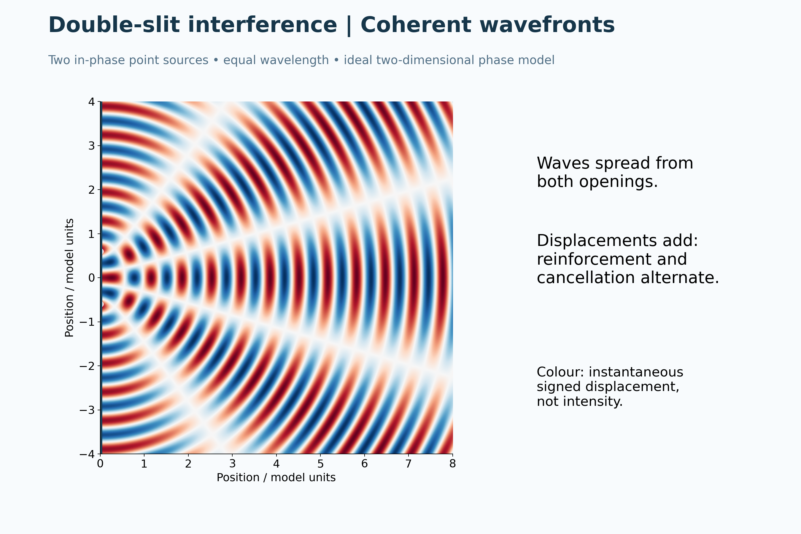
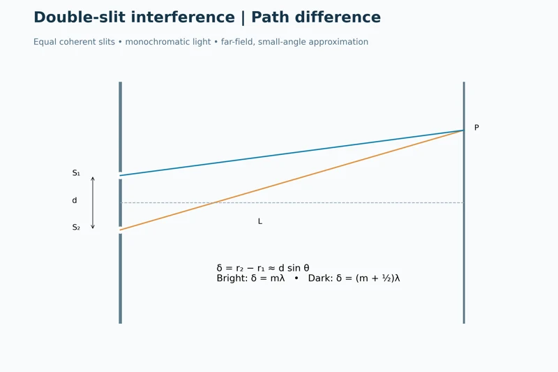
Path difference
A ray diagram relates slit separation, screen geometry and path difference to bright and dark fringes.
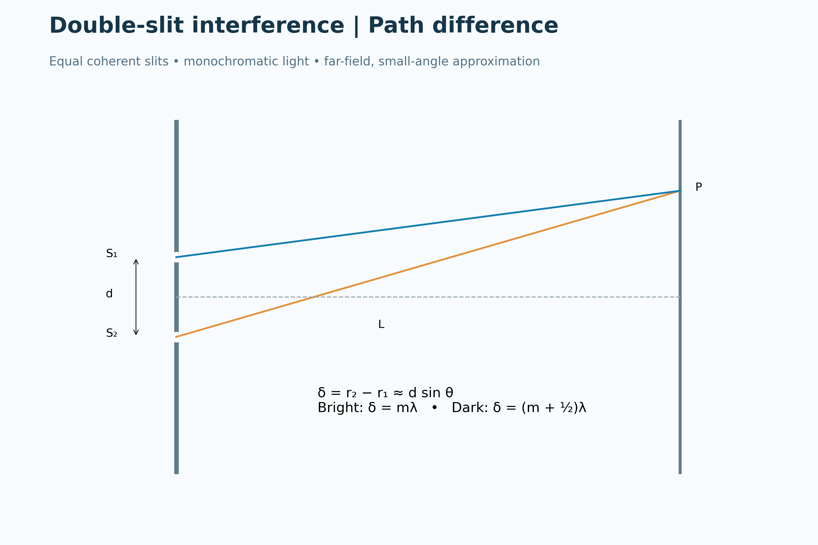

Bright and dark fringes
A relative-intensity curve shows regularly spaced maxima and minima in the narrow-slit approximation.

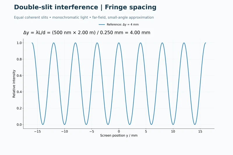
Calculating fringe spacing
A worked example uses 500 nm light, a 2.00 m screen distance and 0.250 mm slit separation to obtain 4.00 mm fringes.

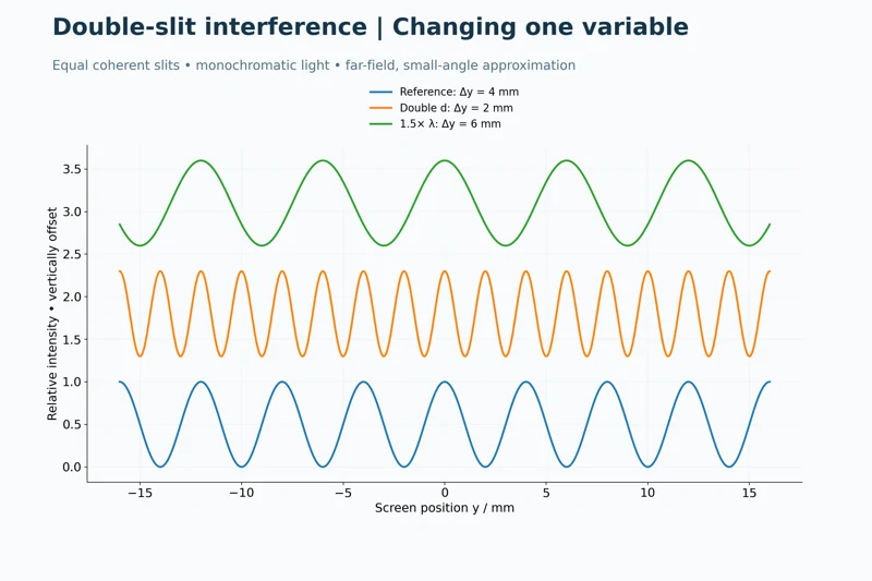
Changing one variable
Offset intensity curves compare the reference pattern with doubled slit separation and increased wavelength.
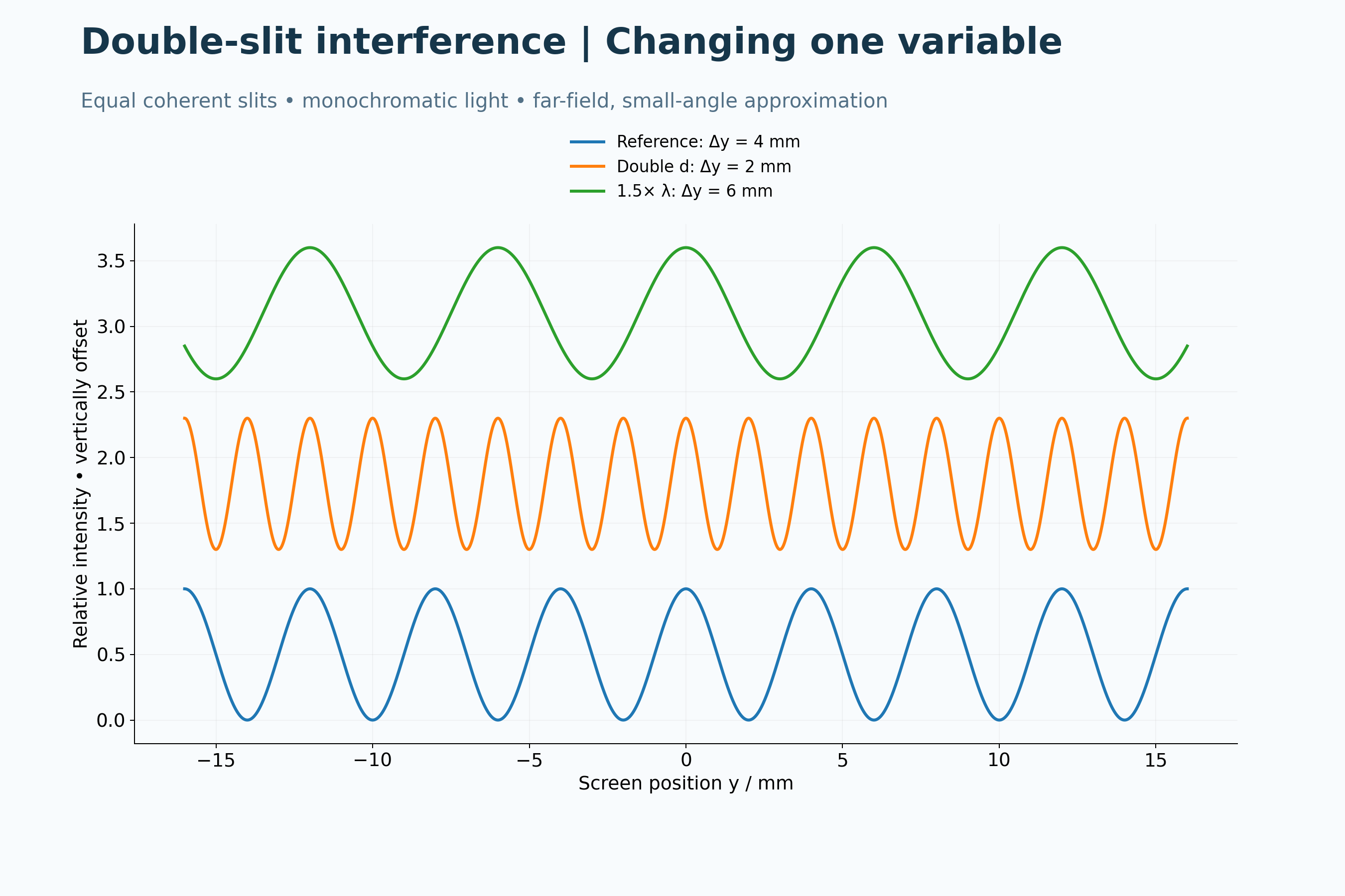
Two-dimensional signed-displacement and far-field narrow-slit models. Colours in the wavefront view are not intensity; the single-slit envelope is neglected.
 PHYSICS · 5 VISUALSWave interference and superpositionFollow two pulses before, during and after overlap using signed displacement.
Constructive superposition
Three snapshots show two positive pulses reinforcing at overlap and then separating.
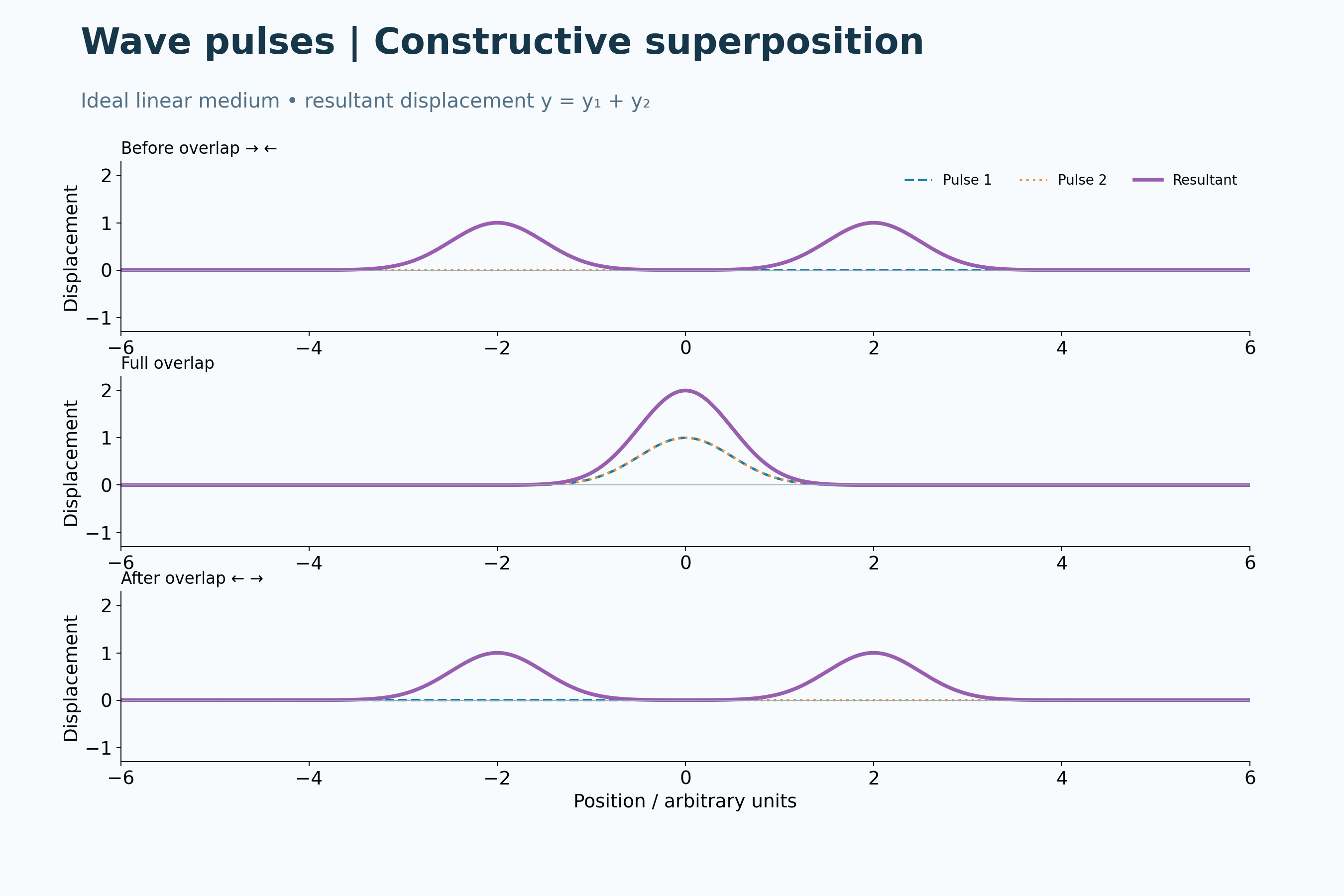
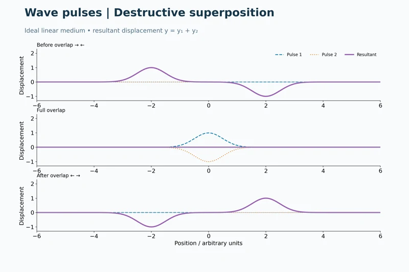
Destructive superposition
Equal positive and negative pulses cancel during complete overlap, then continue moving.


Pulses pass through each other
Before, overlap and after panels show that destructive interference does not destroy the pulses.
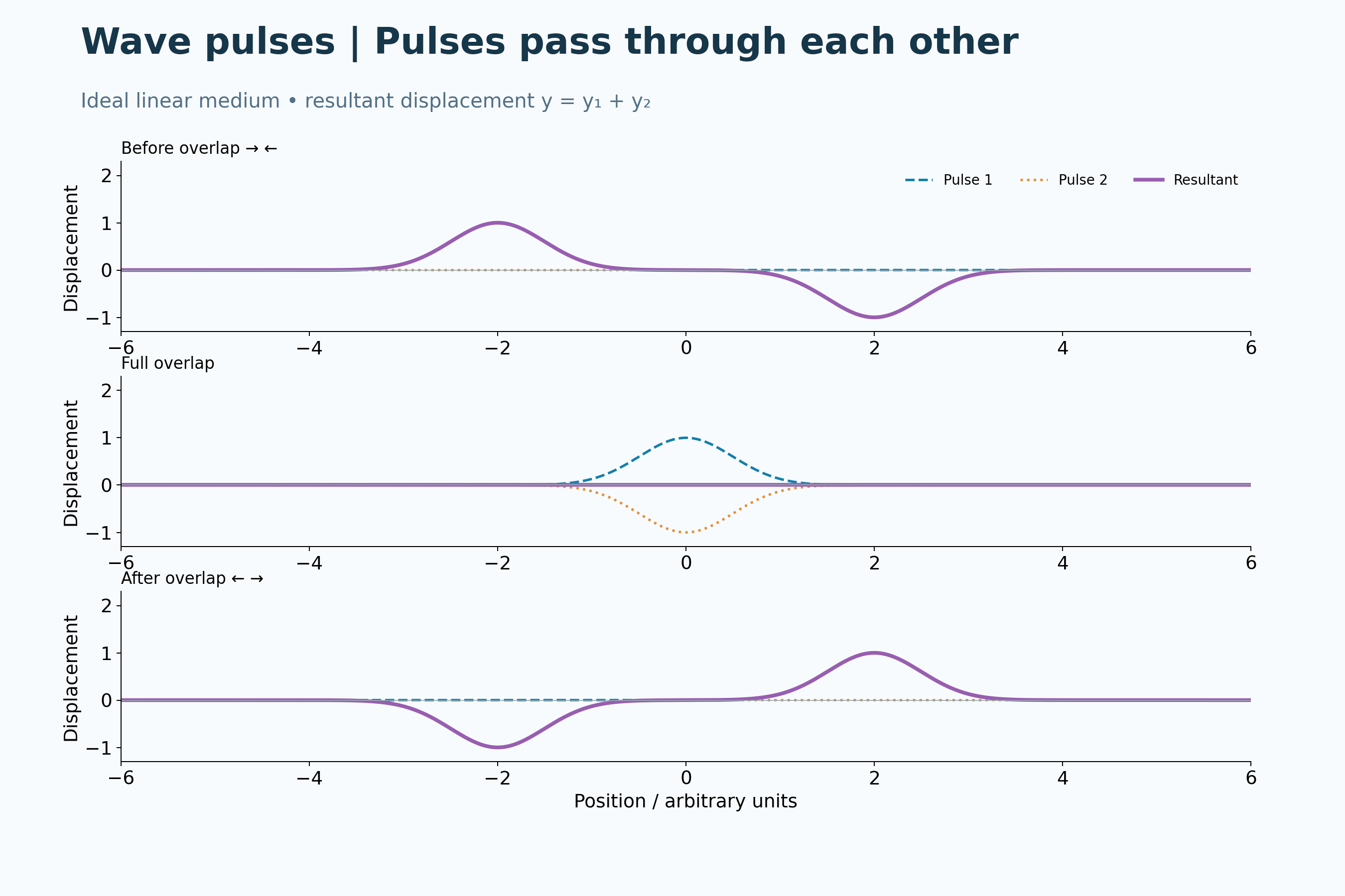

Unequal pulses add point by point
Opposite pulses of unequal size leave a nonzero resultant during overlap.


Displacement is a signed sum
Positive pulses of unequal size combine into a larger resultant and retain their shapes after passing.

Analytical Gaussian pulses in an ideal linear medium, not measured string motion. The resultant is the signed sum of the component displacements.
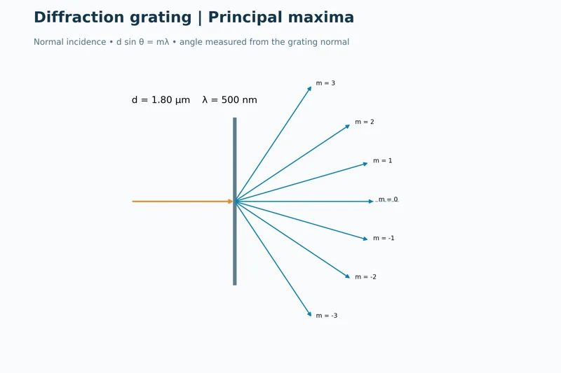 PHYSICS · 5 VISUALSDiffraction gratingUse grating geometry to locate principal maxima and compare wavelengths.
Principal maxima
Rays show positive, zero and negative orders for 500 nm light and 1.80 µm grating spacing.
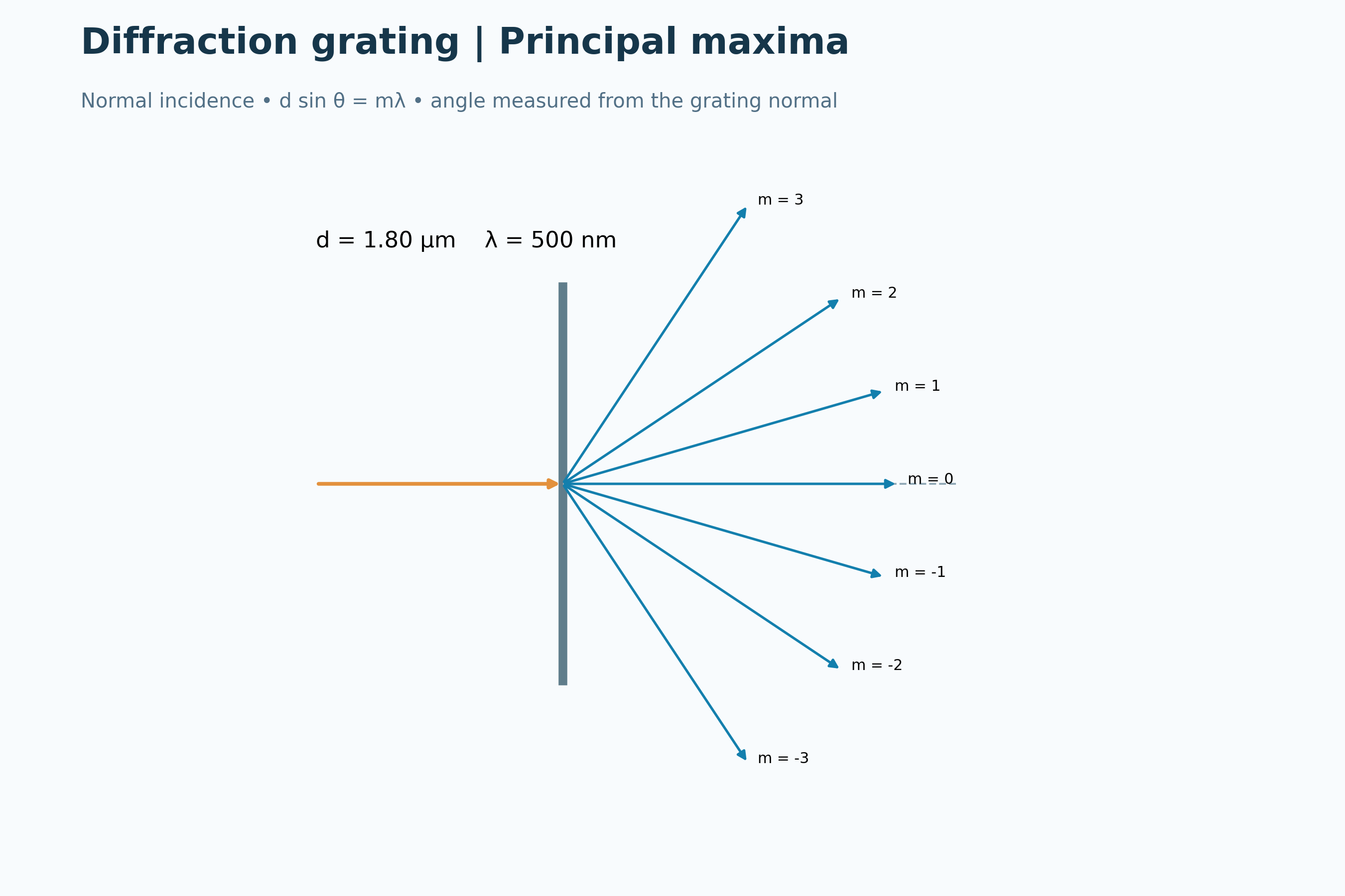
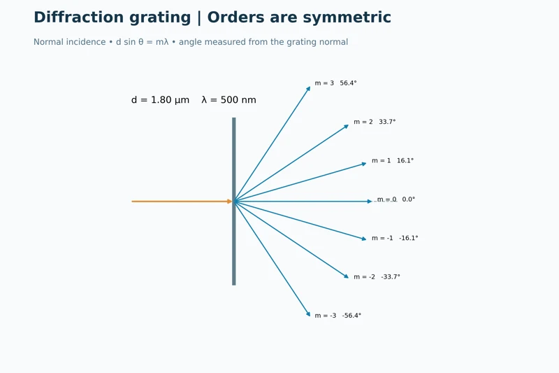
Orders are symmetric
The ray diagram labels matching positive and negative diffraction angles about the central maximum.
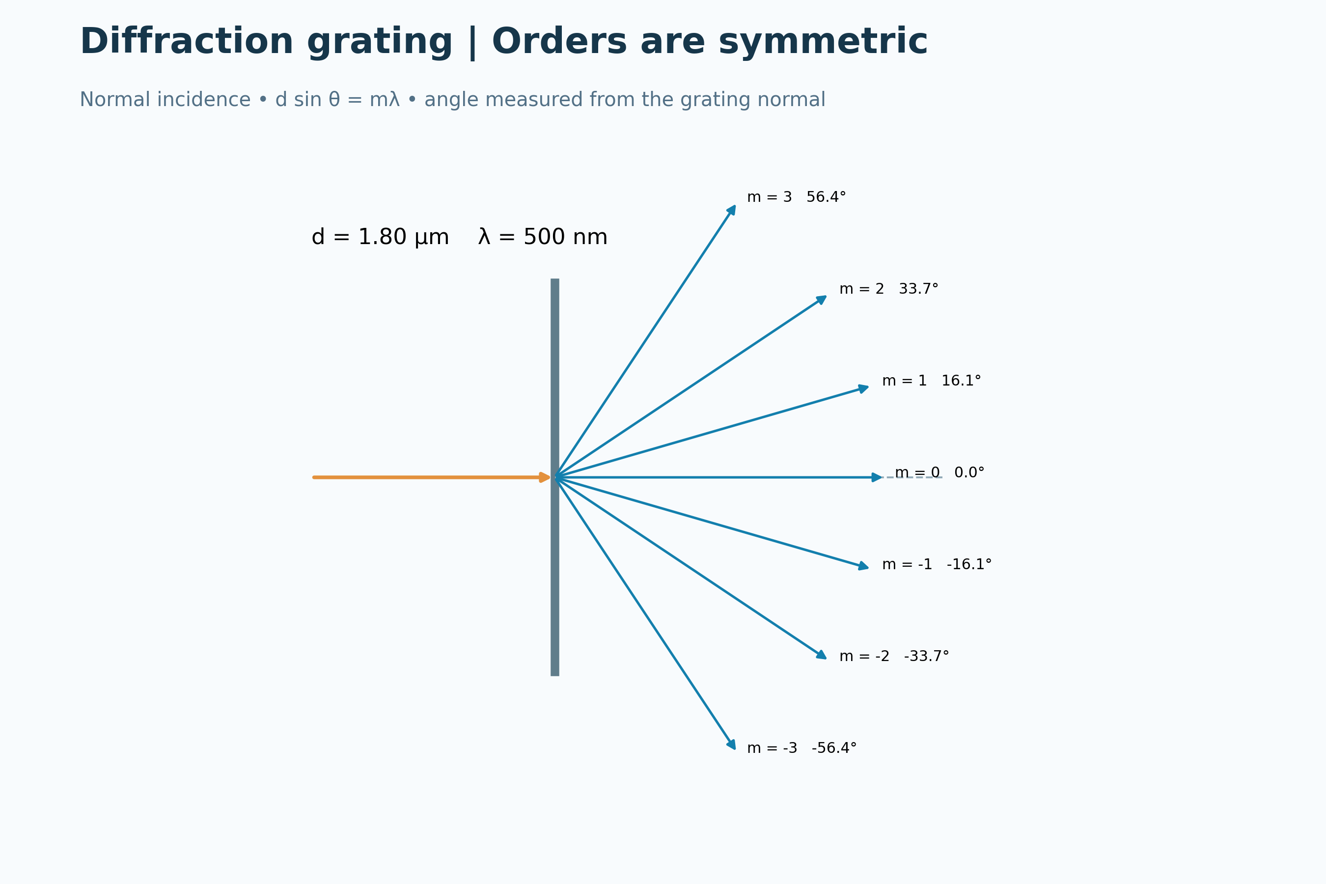
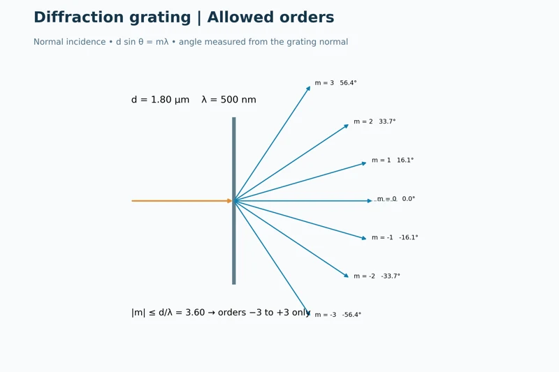
Allowed orders
The condition on the sine limits the example to orders from minus three to plus three.
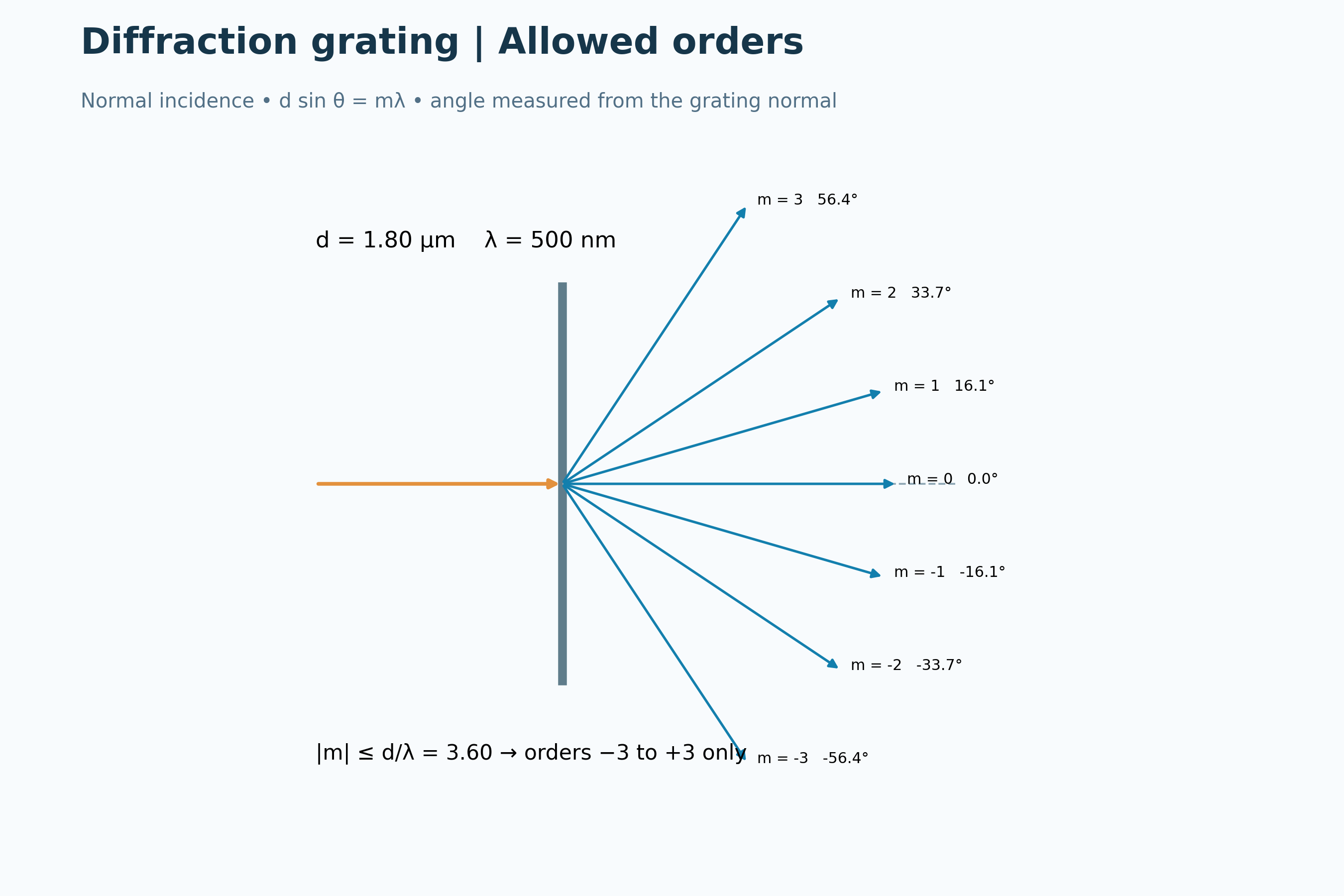

Changing line spacing
Offset position plots compare principal maxima for a reference grating and a smaller line spacing.

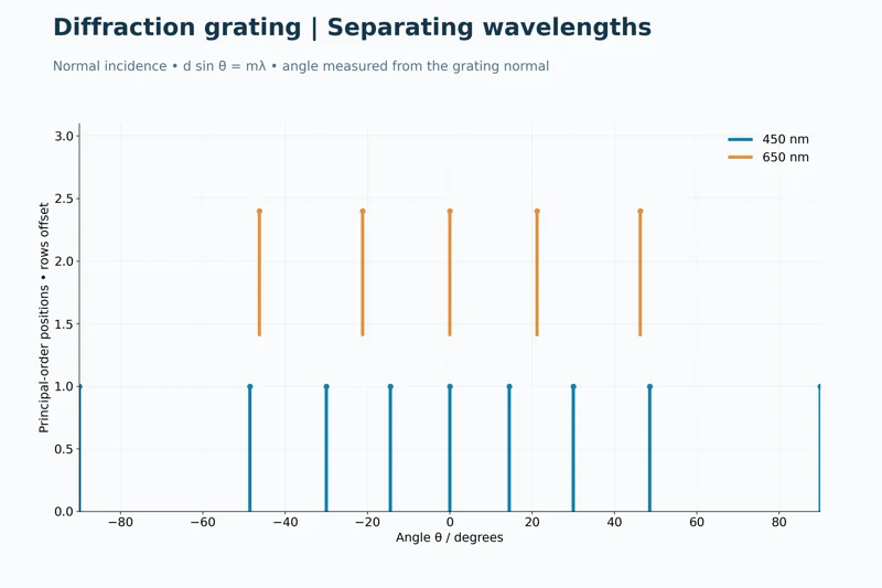
Separating wavelengths
Offset plots compare the angular maxima of 450 nm and 650 nm light.

Normal-incidence grating model using d sin θ = mλ. Plot stems mark angular positions, not relative intensities; grating thickness and finite-width envelopes are omitted.
 PHYSICS · 5 VISUALSDoppler effect and wavefrontsSeparate the effects of source motion and observer motion on sound frequency.
A moving source
Circular wavefronts bunch ahead of a moving source and spread out behind it.


Wavefront spacing
The moving-source diagram adds expressions for wavelengths ahead of and behind the source.


Wavelengths in sound
A numerical example calculates 0.255 m ahead and 0.425 m behind a source moving at 85 m/s.


A moving observer
An approaching observer encounters more crests per second while the wavelength in the medium stays unchanged.


Source motion versus observer motion
Side-by-side examples compare approximately 1333 Hz for source motion with 1250 Hz for observer motion at the same approaching speed.

Classical sound in a stationary medium, with subsonic source motion. Circles are centred on previous source positions; this is not a relativistic light model.
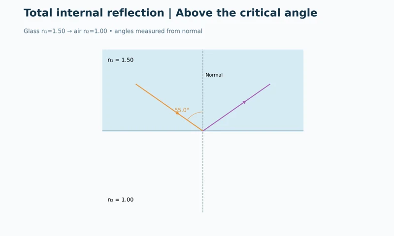 PHYSICS · 5 VISUALSTotal internal reflectionConnect critical angle, refractive index and light guidance in an optical fibre.
Above the critical angle
A glass-to-air ray reflects internally at an incidence angle above the critical angle.


Below, at and above critical
Three ray diagrams compare refraction, a grazing refracted ray and total internal reflection.
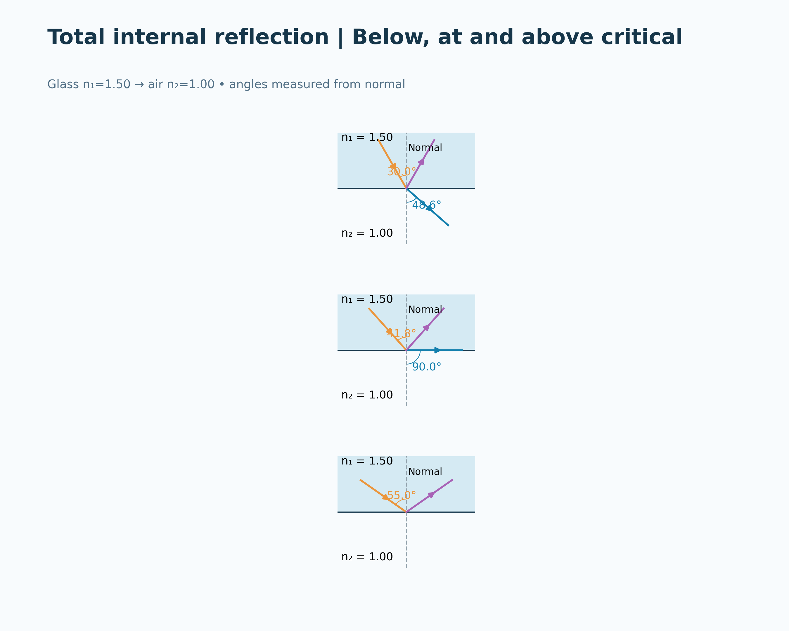

The critical-angle condition
Glass-to-air diagrams accompany sin θc = n2/n1 and a critical angle of approximately 41.81 degrees.


Repeated internal reflection
A ray zigzags along a higher-index core, with 70-degree incidence exceeding the 68.96-degree critical angle.


A higher-index fibre core
A labelled fibre illustration and boundary inset distinguish the protective jacket, cladding and core.

Ideal geometrical-optics models. The fibre is a straight step-index example; evanescent fields and waveguide modes are omitted. The apparatus illustration is not a calibrated cross-section.
 PHYSICS · 5 VISUALSPolarisationConnect transmission-axis angle with the intensity transmitted by ideal polarisers.
Selecting an electric-field direction
A schematic contrasts unpolarised directions over time with one linear polarisation direction.


The angle matters
Three analyser orientations compare transmission fractions of one, one-half and zero.


Malus’ law
A calculated cosine-squared curve relates analyser angle to the fraction of already-polarised incident intensity transmitted.


Keep the two steps separate
Unpolarised input is halved by the first polariser, then reduced to one-eighth by an analyser at 60 degrees.


A middle filter changes transmission
Three ideal polarisers at 0, 45 and 90 degrees transmit one-eighth of the initially unpolarised input.
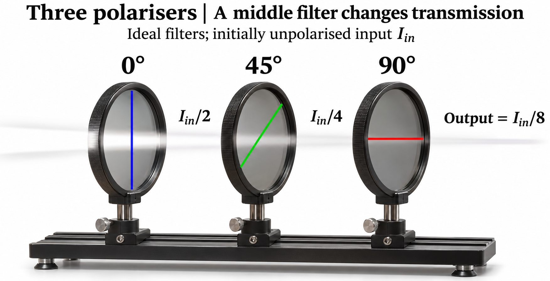
Ideal-filter models and an illustrative apparatus view, not measured filter efficiencies. Electric-field directions are shown perpendicular to propagation.
 PHYSICS · 5 VISUALSCapacitance and stored energyExplore separated charge, parallel-plate geometry and energy stored in a capacitor.
Separated charge
Parallel plates carry equal and opposite charge with an air gap between them.


The central electric field
A schematic shows a uniform field from the positive plate to the negative plate and E ≈ V/d.
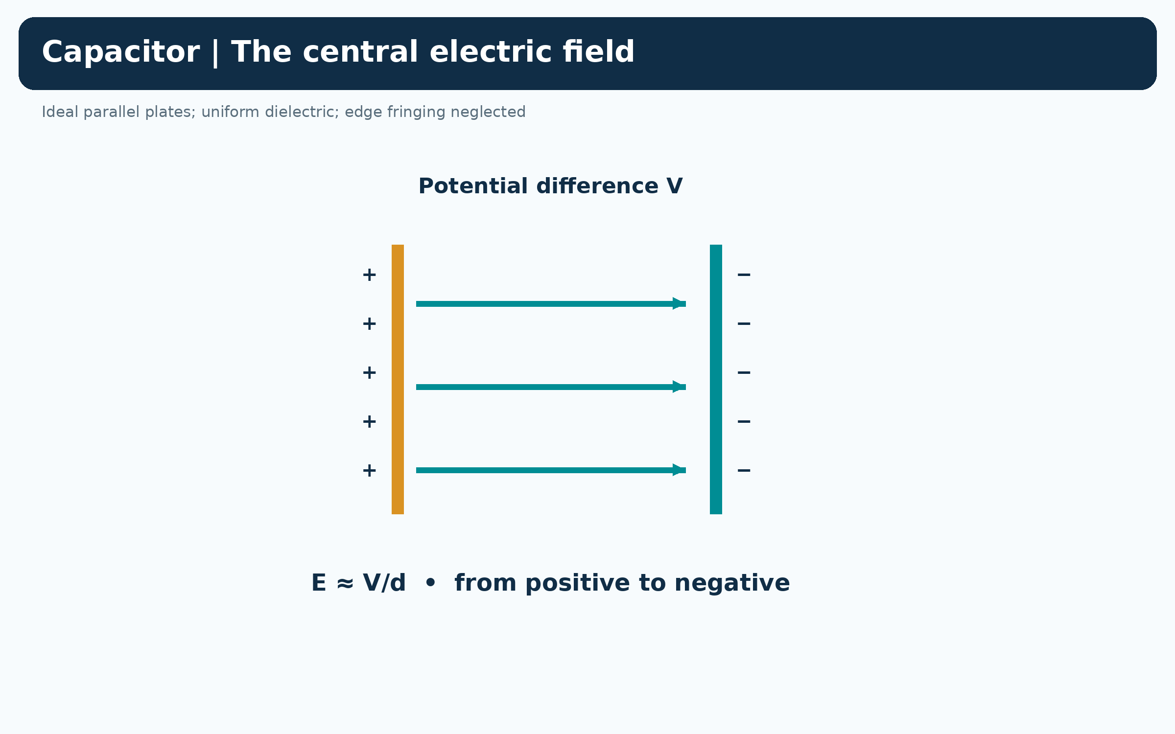

Geometry sets the capacitance
Three cases compare a reference capacitor with doubled separation and doubled plate area.

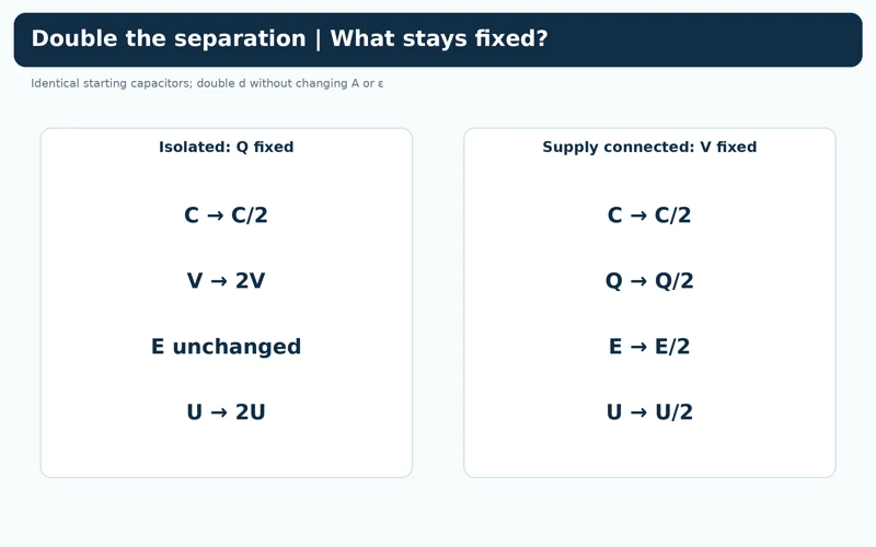
What stays fixed?
A comparison lists changes in capacitance, voltage, charge, field and stored energy when separation doubles at fixed charge or fixed voltage.
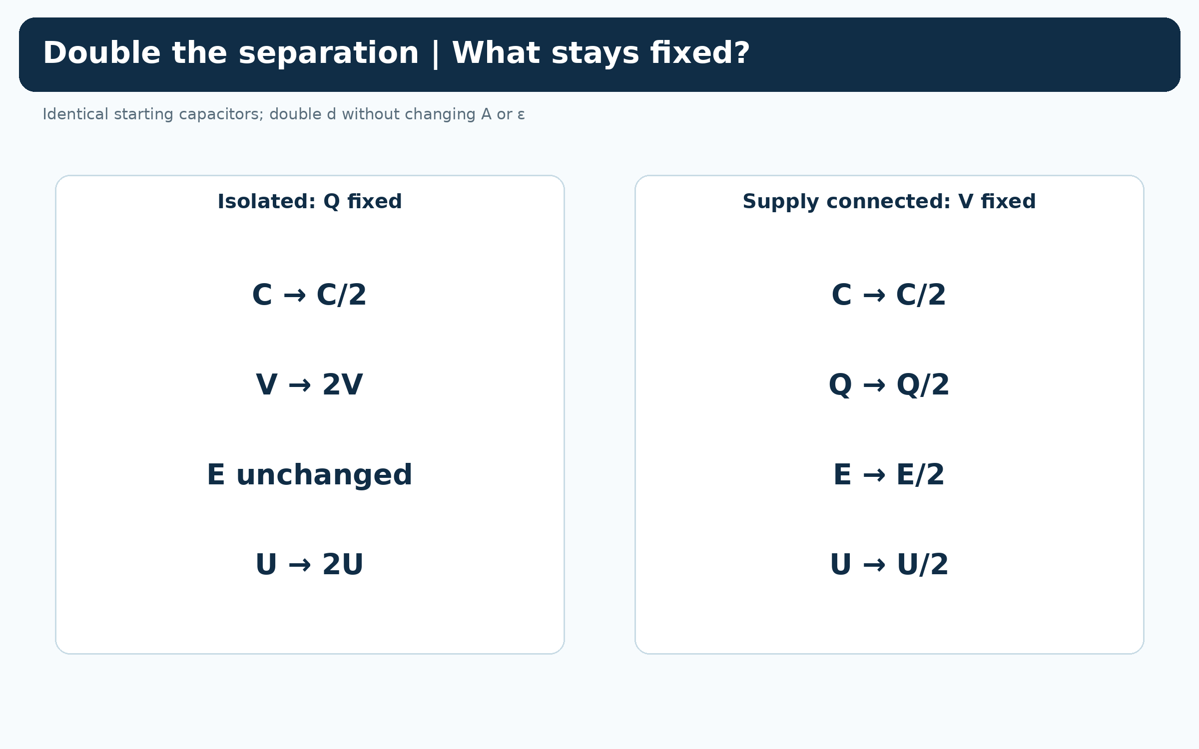

Charge, voltage and energy
A 100 µF capacitor at 12 V stores 1.20 mC of charge and 7.20 mJ of energy.

Ideal parallel plates with a uniform dielectric; edge fringing is neglected. Three-dimensional plates are illustrative rather than a finite-field simulation.
 PHYSICS · 5 VISUALSRC charging and dischargingRead exponential changes in capacitor voltage, charge and current.
Voltage builds gradually
A charging curve approaches the supply voltage with a time constant of one second.


Voltage, charge and current
Aligned plots show rising capacitor voltage and charge while charging-current magnitude falls.


Stored energy leaves the capacitor
Discharge plots show capacitor voltage, charge and current magnitude decreasing exponentially.


One time constant
Normalised curves mark 0.632 of final voltage during charging and 0.368 of initial voltage during discharging.

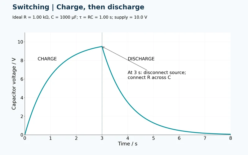
Charge, then discharge
A continuous voltage curve changes from charging to discharging when the source is disconnected at three seconds.

Calculated ideal RC curves for R = 1.00 kΩ, C = 1000 µF and a 10.0 V source. Parasitic circuit effects are omitted; current plots show magnitude.
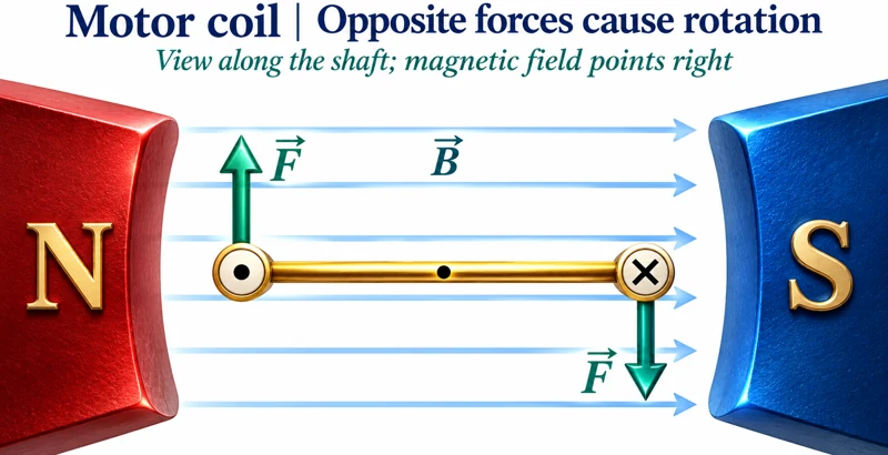 PHYSICS · 5 VISUALSElectric motor principleConnect forces on a current loop with torque, commutation and energy transfer.
Opposite forces cause rotation
An end-on coil between magnetic poles shows opposite current directions and a clockwise force couple.
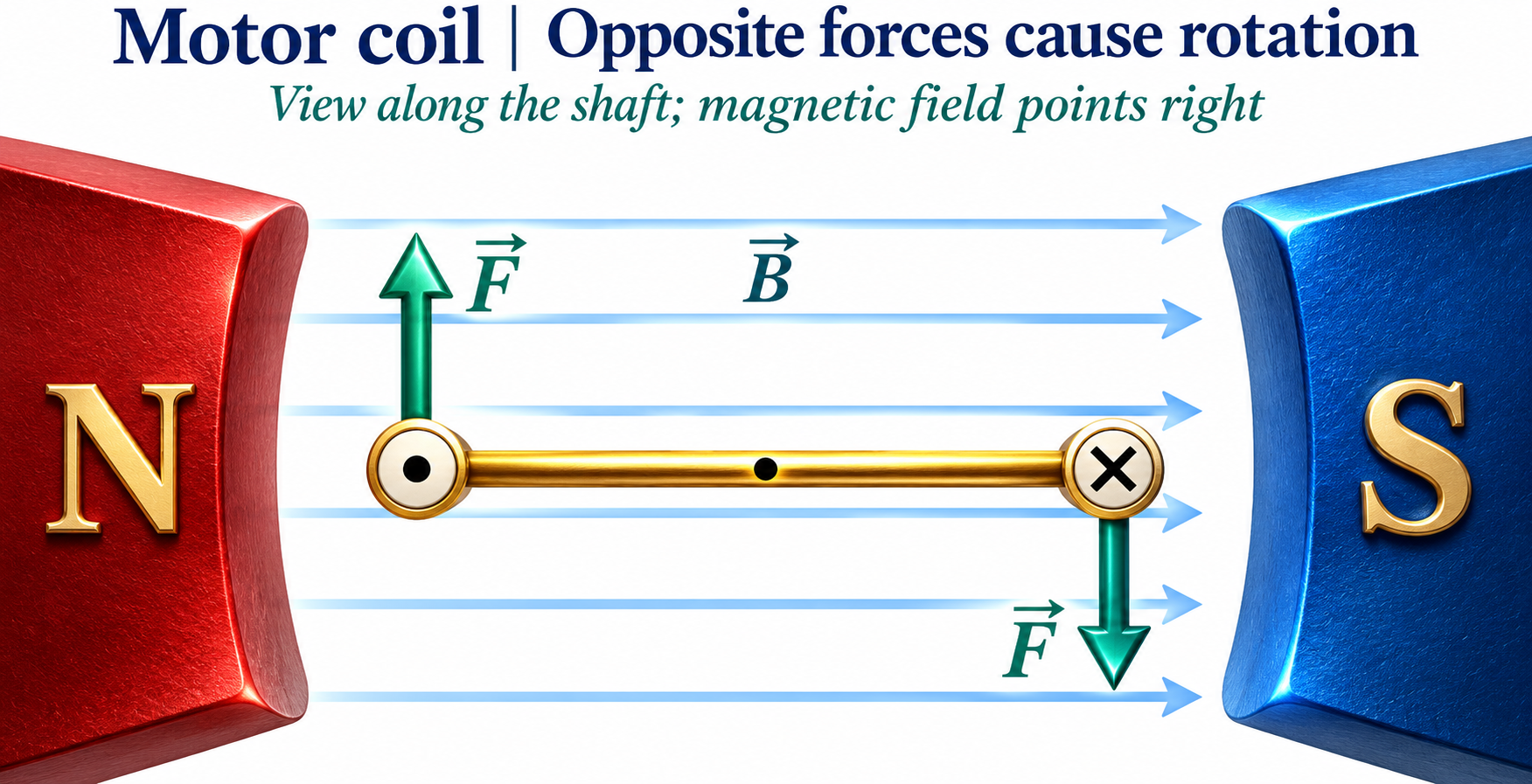

Applying the magnetic-force rule
A rightward field gives an upward force on the left current and a downward force on the right current.


Torque through a rotation
An ideal commutated torque-magnitude curve varies with the coil-width angle to the field.


Reverse current each half-turn
Four coil positions show how current reversal maintains clockwise torque through the rotation.
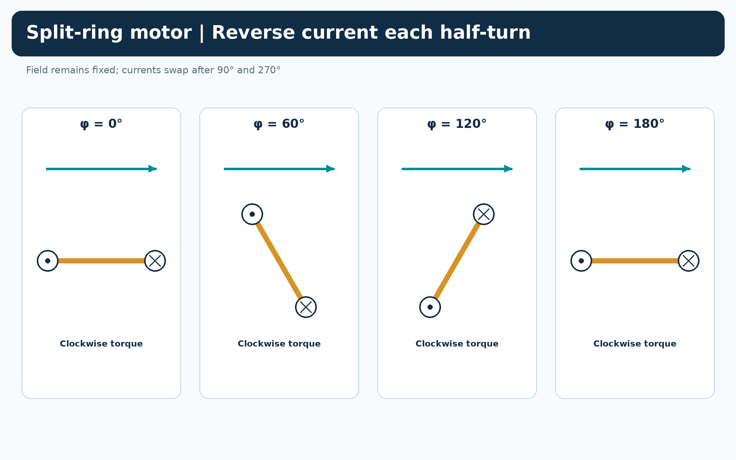

Following the energy
A motor diagram separates electrical input, useful rotational output and heat and friction losses.

Ideal end-on coil diagrams with instantaneous commutation; dead zones and detailed mechanical construction are omitted. The torque graph defines φ as the coil-width angle to the field, not the normal angle.
 PHYSICS · 5 VISUALSTransformer principleConnect changing magnetic flux, turns ratio, voltage and current in transformers.
Changing core flux
Separate primary and secondary windings share a laminated iron core carrying changing magnetic flux.


Stepping voltage up
A 100-to-500 turns example increases 12 V rms to 60 V rms in an ideal transformer.

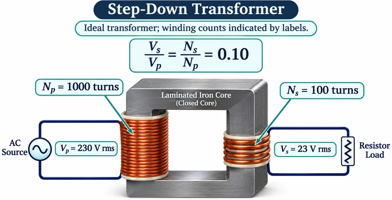
Stepping voltage down
A 1000-to-100 turns example reduces 230 V rms to 23 V rms.


Ideal power balance
A worked example balances 12 V at 2.0 A with 60 V at 0.40 A, both 24 W.

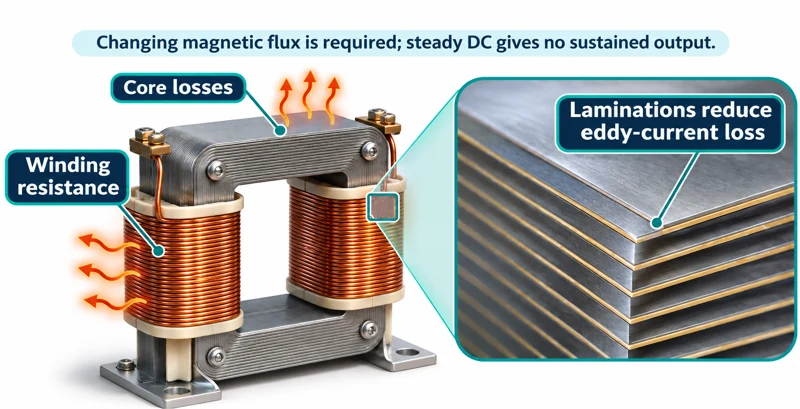
Real losses and laminations
A transformer illustration labels winding resistance, core losses and laminations that reduce eddy-current loss.

Illustrative transformer geometry with symbolic windings; labelled turn counts are not literal visible coil counts. Numerical examples use ideal transformers and rms quantities with a resistive load.
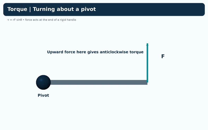 PHYSICS · 5 VISUALSTorque and perpendicular lever armExplain turning effect using force, direction and perpendicular distance from a pivot.
Turning about a pivot
An upward force on the right end of a handle produces anticlockwise torque.
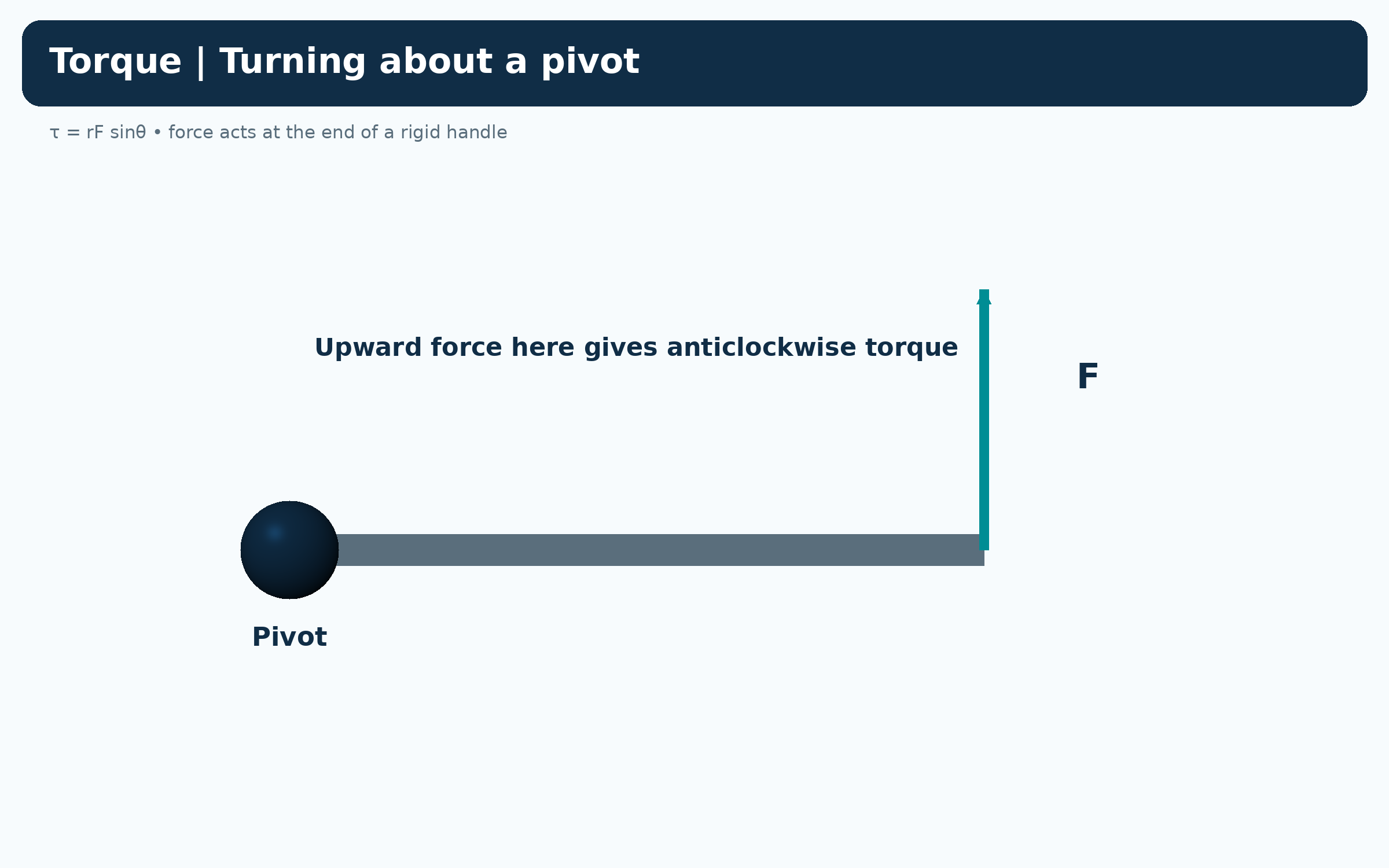
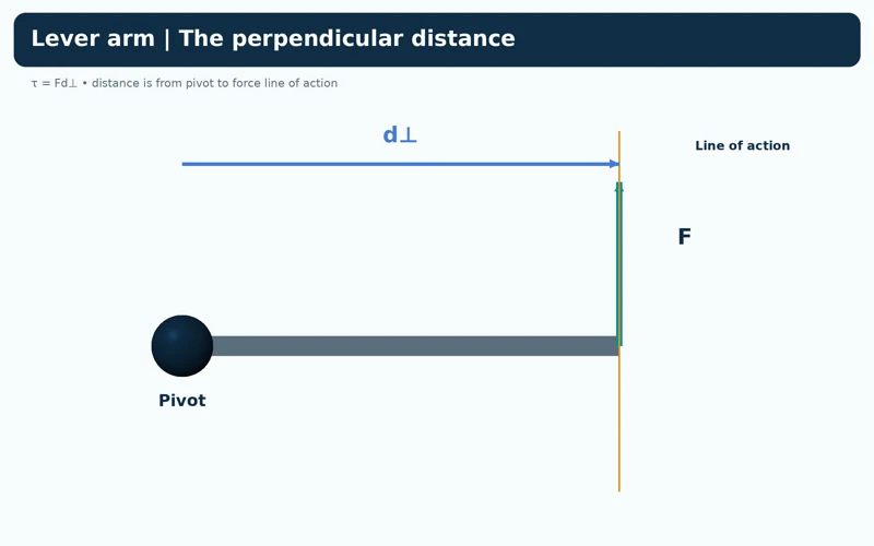
The perpendicular distance
A diagram marks the shortest distance from the pivot to the force’s line of action.


Force angle changes torque
The same 10 N force at 90, 30 and zero degrees produces 2.0, 1.0 and zero newton metres.


A longer lever
A perpendicular 10 N force gives 1.0 N m at 0.10 m and 2.0 N m at 0.20 m.


Clockwise and anticlockwise signs
A downward end force is clockwise and negative under the stated sign convention.

Rigid-handle schematics using τ = rF sin θ. Signed torque examples explicitly take anticlockwise as positive.
 PHYSICS · 5 VISUALSKinetic model and gas pressureLink molecular motion and wall collisions with gas pressure and temperature.
Constant random motion
A rigid-container illustration shows gas particles moving in different directions.
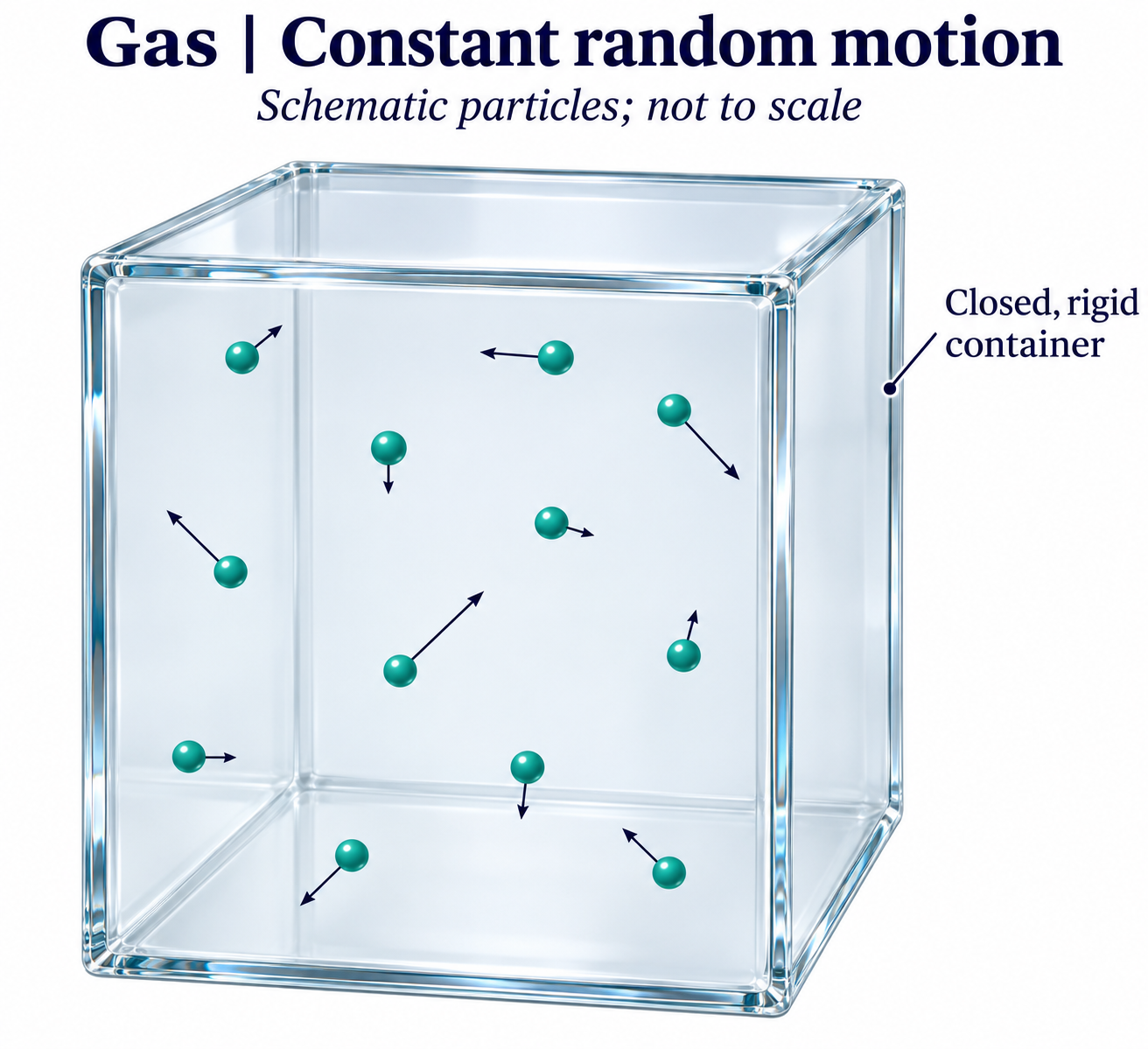
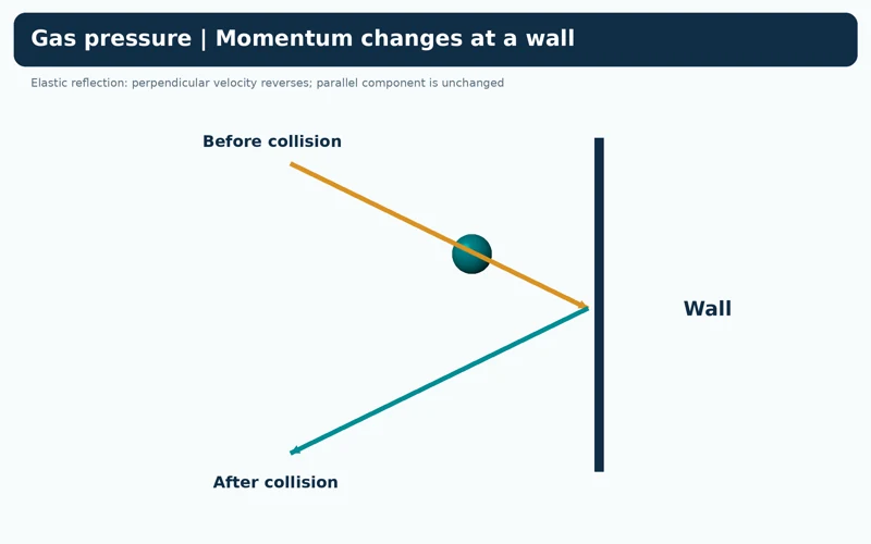
Momentum changes at a wall
An elastic collision reverses the velocity component perpendicular to the wall while retaining the parallel component.
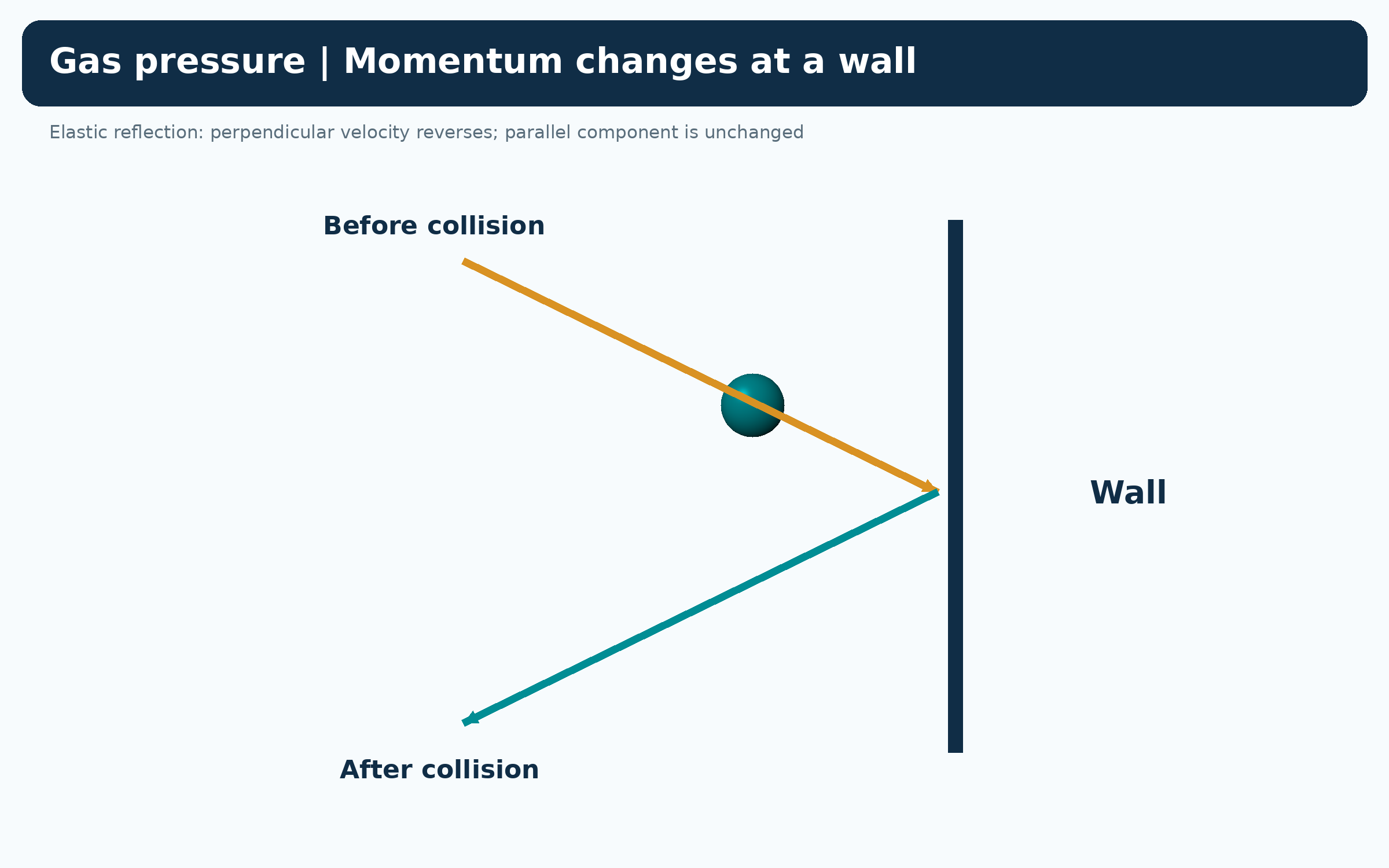

Heating broadens the distribution
Calculated speed distributions at 300 K and 600 K compare the same molecular mass.


Same particles, faster motion
Equal-size containers with equal particle counts compare motion at 300 K and 600 K.
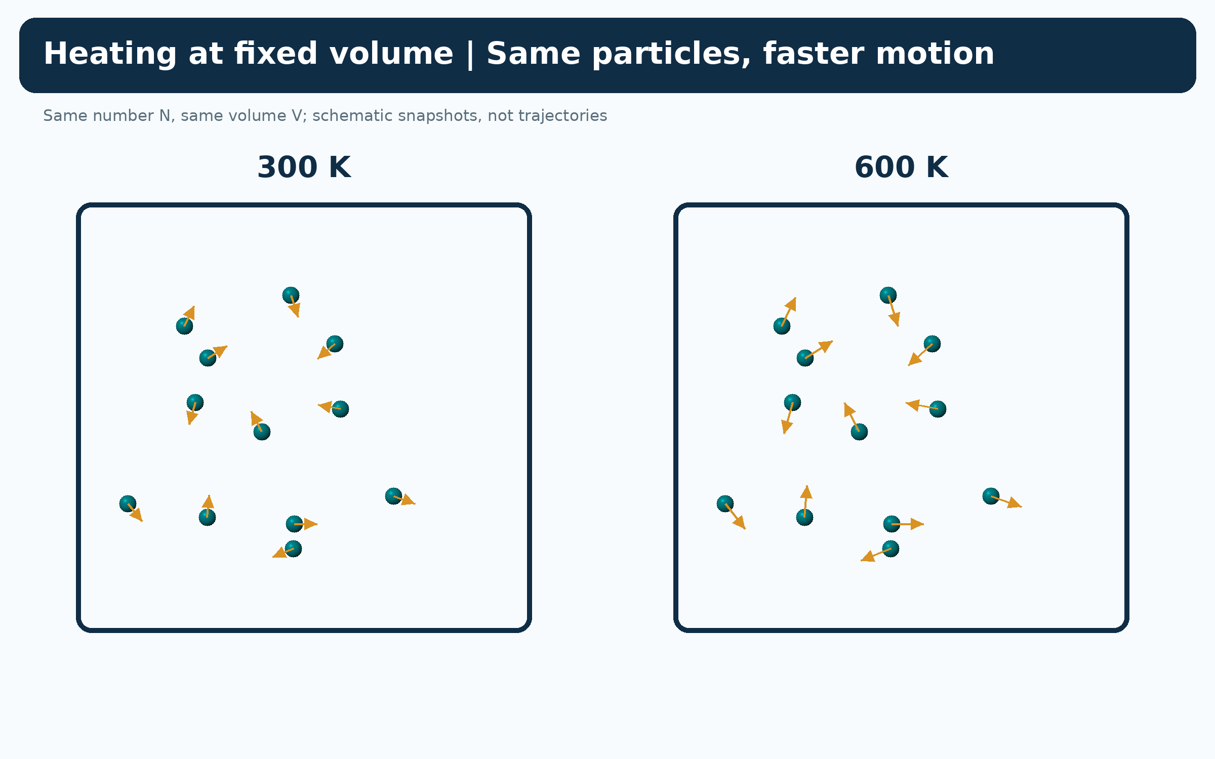

Temperature and pressure
A fixed-volume comparison connects doubled absolute temperature with doubled ideal-gas pressure.
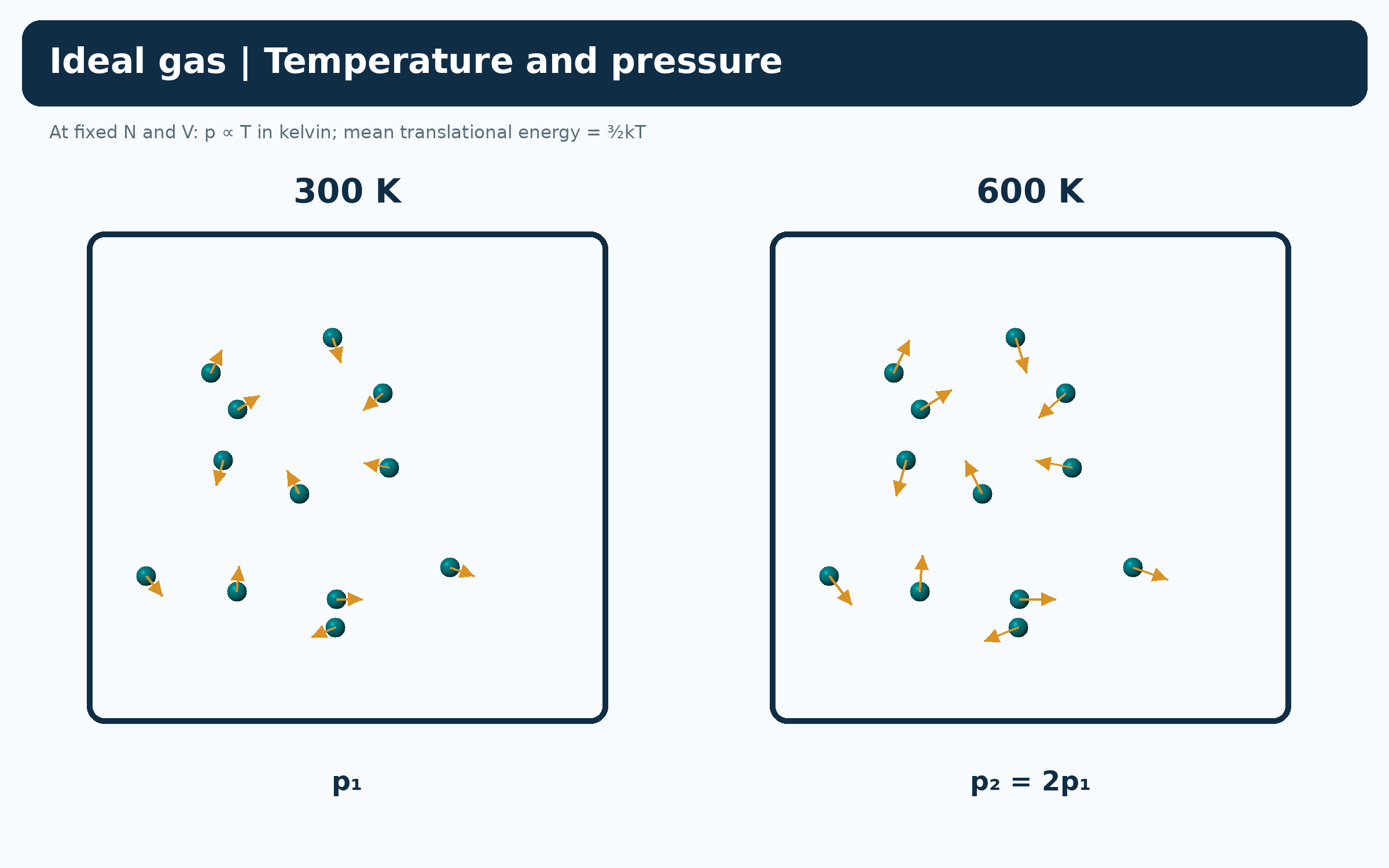
Ideal-gas schematics and calculated Maxwell–Boltzmann speed distributions. Particles are not to physical scale and snapshots are not molecular-dynamics trajectories.
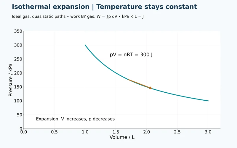 PHYSICS · 5 VISUALSPressure-volume gas processesRead gas processes and work from pressure-volume diagrams.
Isothermal expansion
An ideal-gas isotherm with pV = 300 J shows pressure decreasing as volume increases.


Three process constraints
Side-by-side plots compare isothermal, isobaric and isochoric paths.

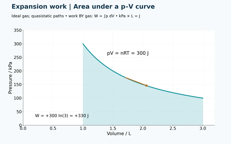
Area under the curve
A shaded isothermal expansion from one to three litres gives approximately +330 J of work by the gas.
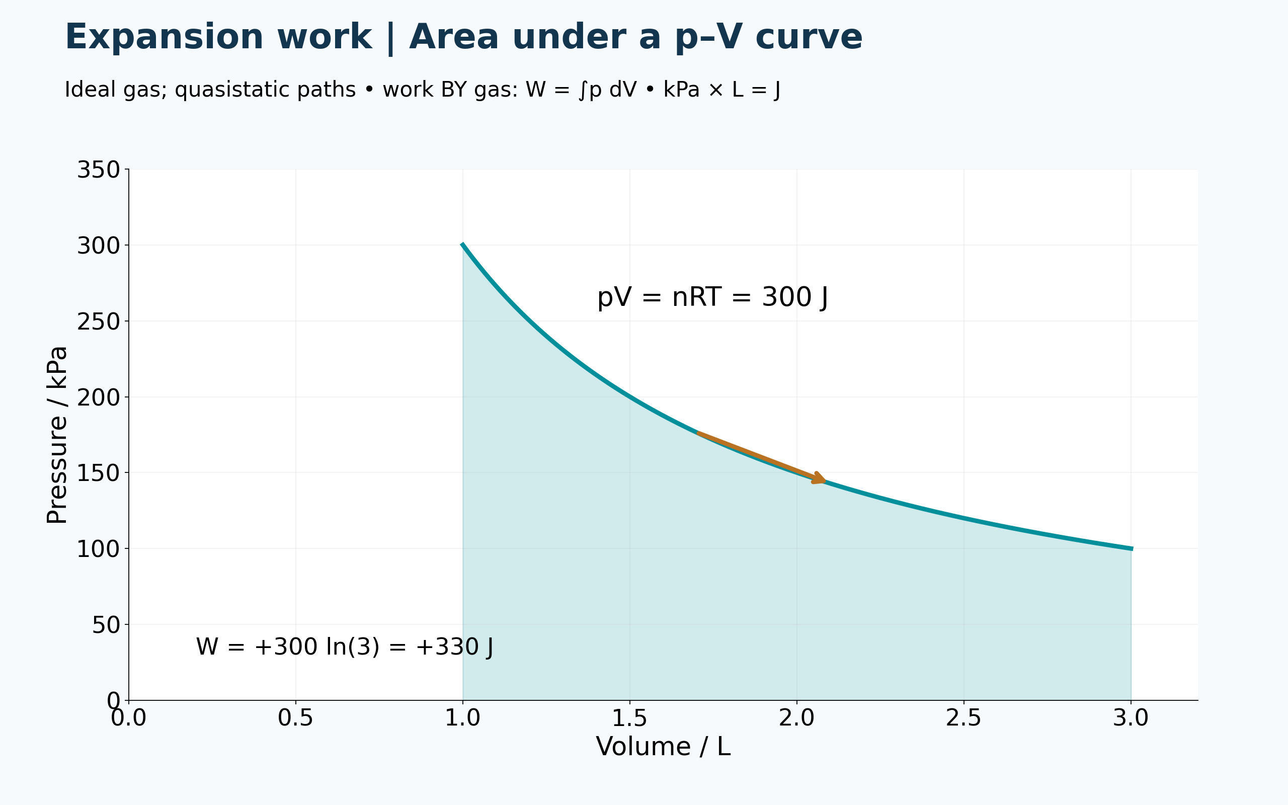

Compression changes the sign
The reverse isothermal path gives approximately −330 J of work by the gas.

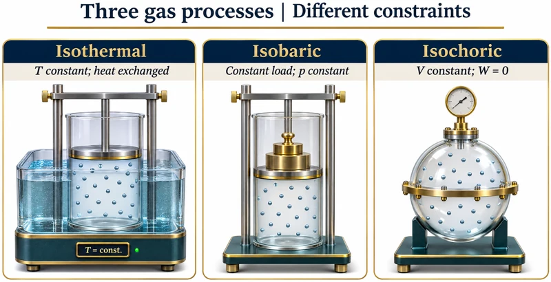
Apparatus for three processes
Illustrations compare a temperature-controlled piston, a constant-load piston and a rigid vessel.
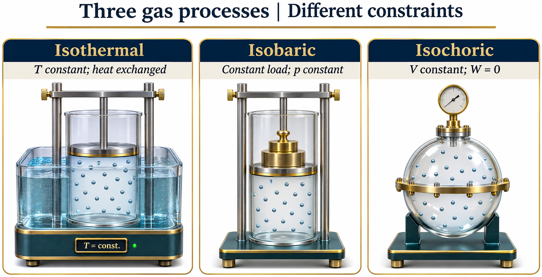
Quasistatic ideal-gas paths; work is defined as work done by the gas. Apparatus illustrations are conceptual, not experimental measurements.
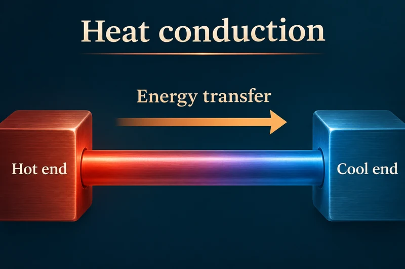 PHYSICS · 5 VISUALSHeat conductionConnect energy transfer through solids with temperature difference, material and geometry.
Energy moves from hot to cool
A rod between hot and cool ends shows the direction of net energy transfer.


Vibrations about fixed sites
A lattice inset illustrates energy transfer through vibrations without bulk movement of the solid.
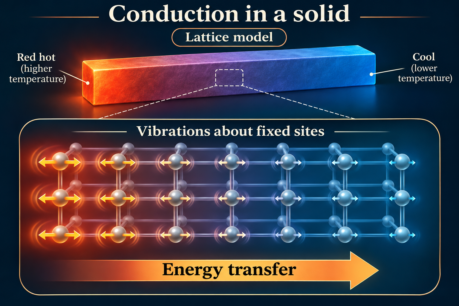

Steady-state transfer through a rod
A labelled rod shows cross-sectional area, length and end temperatures alongside the conduction-rate equation.
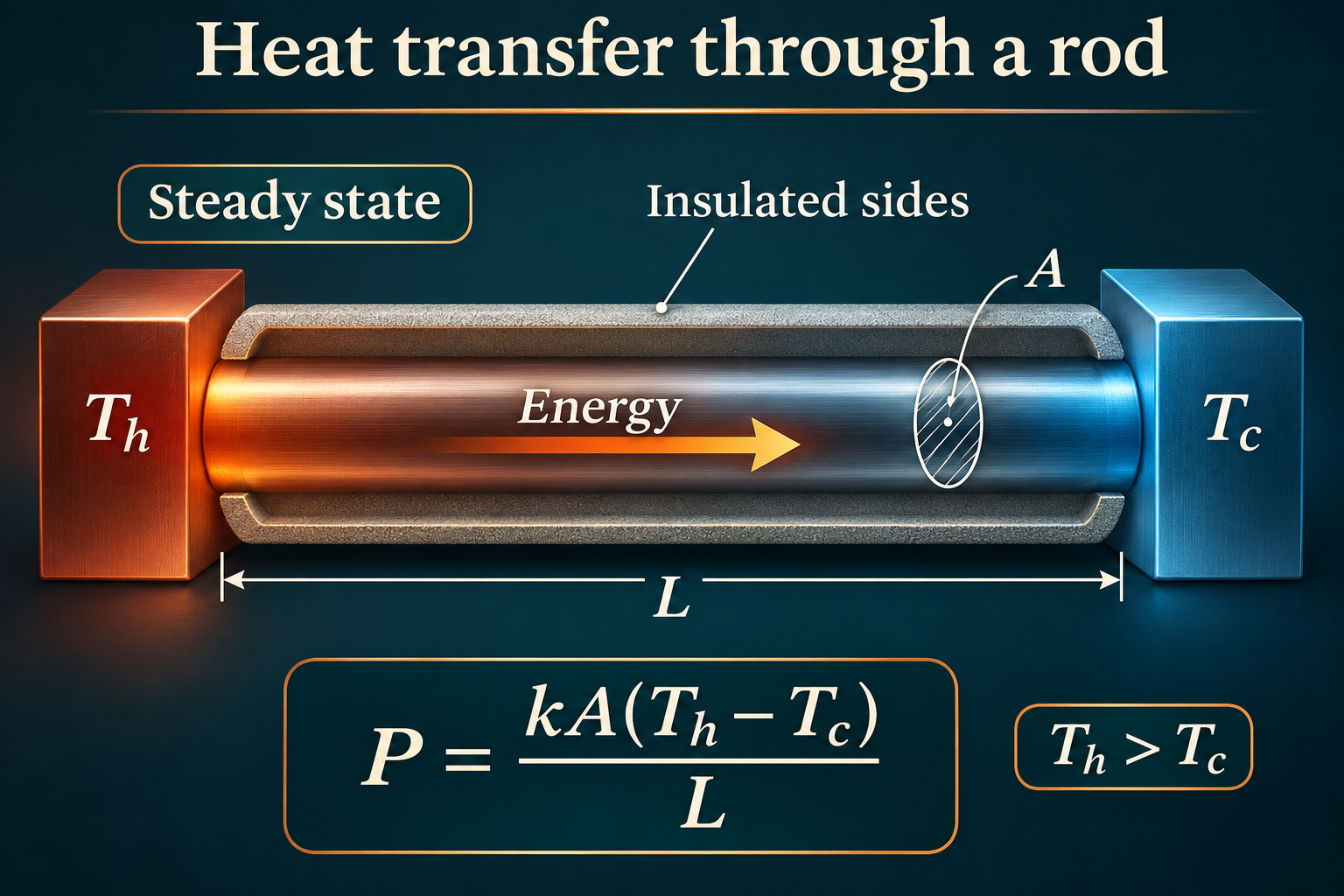
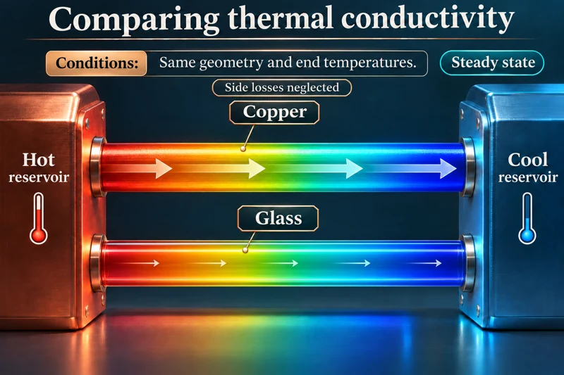
Comparing thermal conductivity
Copper and glass rods with the same geometry and end temperatures illustrate different rates of conduction.
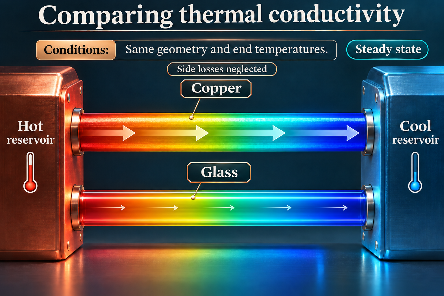

How metals conduct energy
A microscopic inset combines lattice vibrations and mobile electrons in a metal conductor.

Qualitative false-colour illustrations, not measured thermography or atomic coordinates. The rod equation assumes steady state, uniform conductivity and negligible side losses; metal conduction includes electronic and lattice contributions.
 PHYSICS · 5 VISUALSConvection and radiationDistinguish heat transfer through matter from radiation that can cross a vacuum.
Three ways energy transfers
A spoon, heated water and the Sun–Earth example compare conduction, convection and radiation.


Convection in water
A tank diagram shows warm water rising and cooler water sinking between warmer and cooler boundaries.

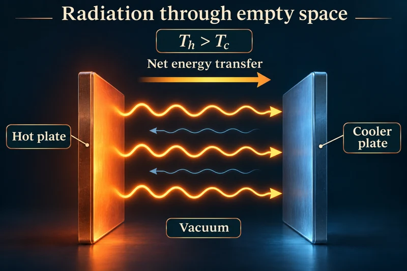
Radiation through empty space
Two plates exchange radiation across a vacuum, with net energy transfer from hotter to cooler.


A heated container
A cutaway distinguishes conduction through the base, convection in water and radiation from surfaces.
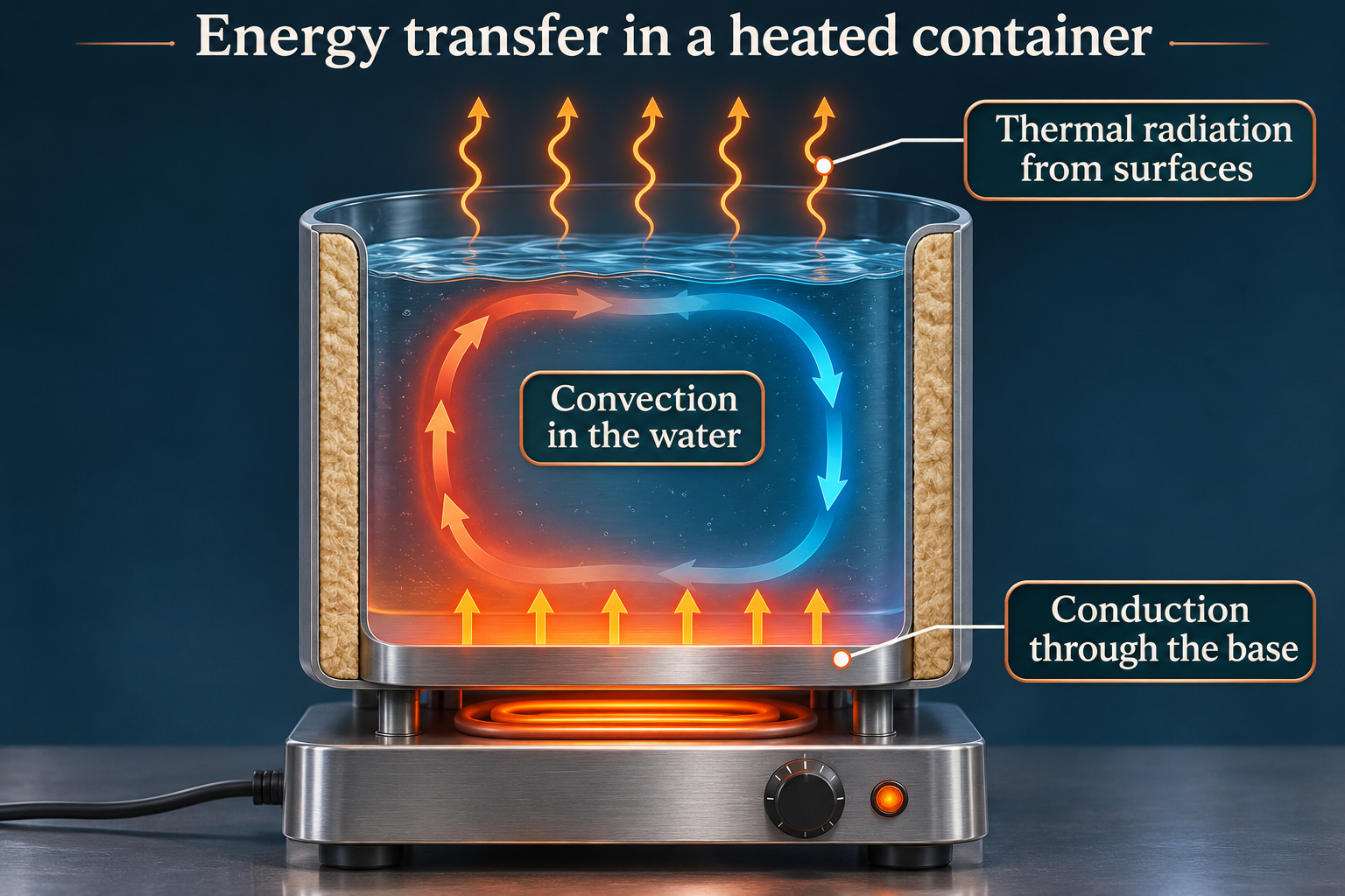

Heating a room
A radiator scene distinguishes metal conduction, circulating air and electromagnetic radiation.
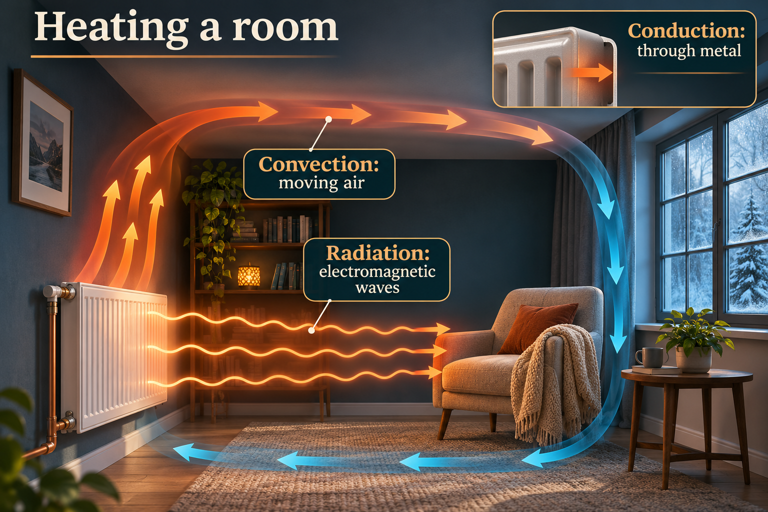
Qualitative circulation, surface-radiation and false-colour illustrations, not computational fluid dynamics or thermography. Radiation exchange is bidirectional; net transfer is from hotter to cooler.
 PHYSICS · 5 VISUALSHeating curves and latent heatSeparate temperature rises from phase changes on an energy-input graph.
Melting without a temperature rise
An energy-input graph follows warming ice, a melting plateau and warming liquid water.
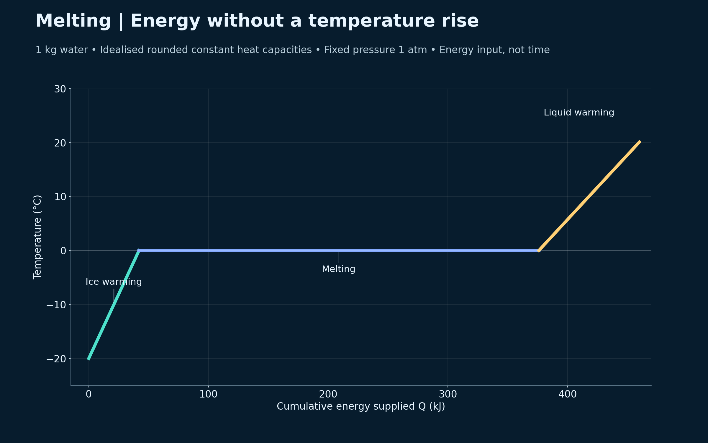
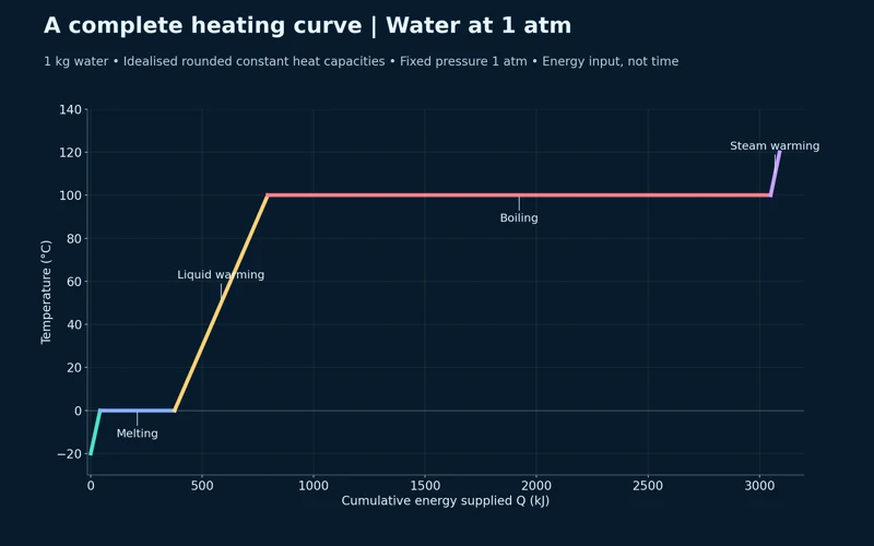
A complete heating curve
The water curve includes melting at zero degrees Celsius, boiling at 100 degrees Celsius and warming steam.

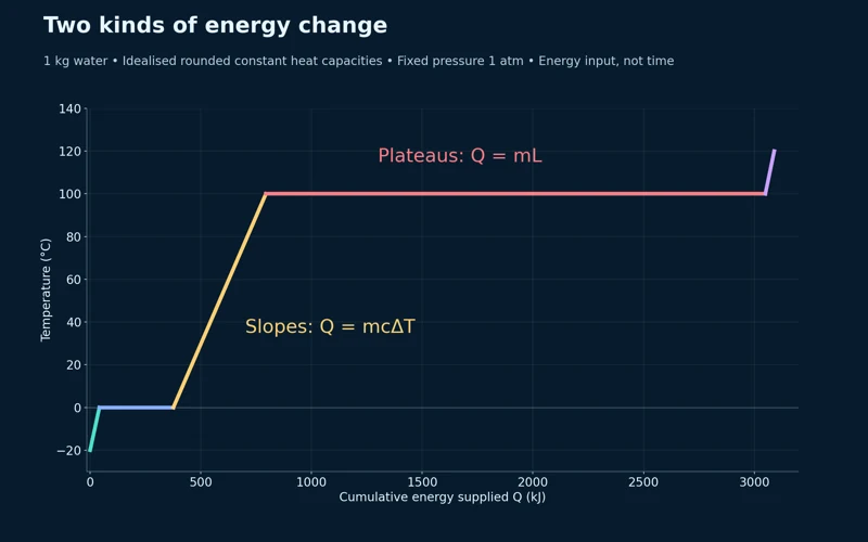
Two kinds of energy change
The graph distinguishes Q = mcΔT on sloping sections from Q = mL during phase changes.

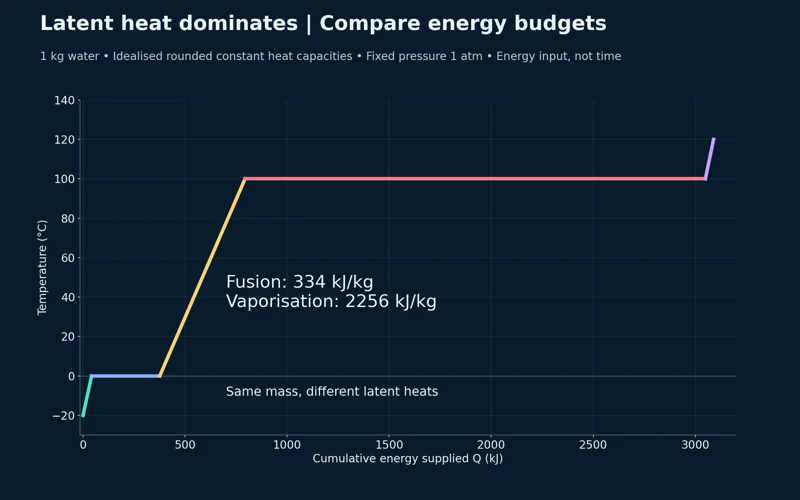
Comparing latent heats
The same water mass requires 334 kJ/kg for fusion and 2256 kJ/kg for vaporisation in the model.


Where the energy goes
A stage-energy bar chart compares warming ice, melting, warming water, boiling and warming steam, totalling 3090 kJ.

Idealised one-kilogram water model at one atmosphere, using rounded constant heat capacities and latent heats. The horizontal axis is cumulative energy supplied, not elapsed time.
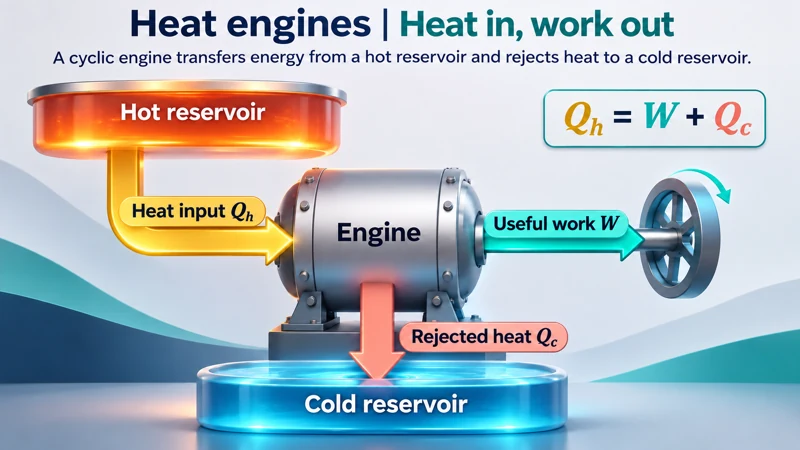 PHYSICS · 5 VISUALSHeat engine energy balanceAccount for heat input, useful work and rejected heat in a cyclic engine.
Heat in, work out
An engine illustration connects hot and cold reservoirs with heat input, useful work and rejected heat.
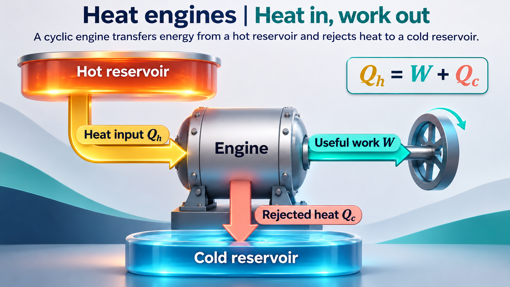

Every joule accounted for
A flow diagram divides 1000 J input into 300 J work and 700 J rejected heat.


Work divided by heat input
The same energy balance gives an efficiency of 30 percent.

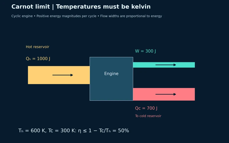
The Carnot limit
Reservoir temperatures of 600 K and 300 K give a maximum possible efficiency of 50 percent.
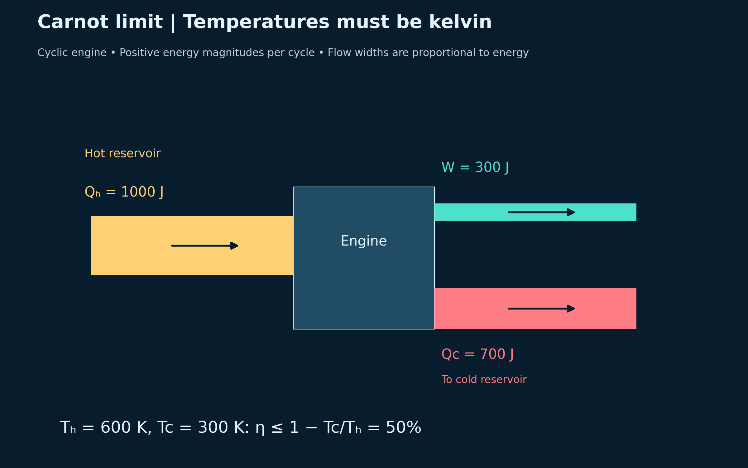
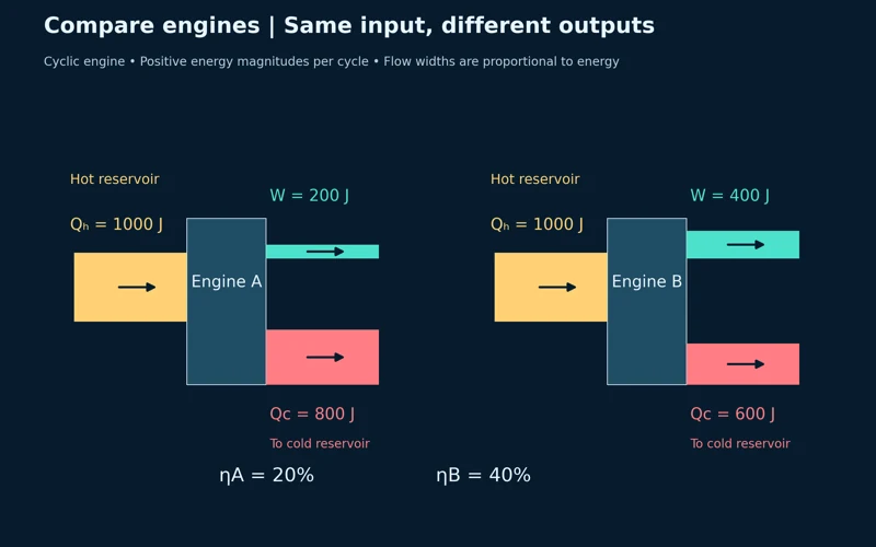
Same input, different outputs
Two engines with 1000 J input compare 20 percent and 40 percent efficiency.

Cyclic-engine energy balances with positive heat and work magnitudes. Flow widths are proportional to energy; the Carnot expression gives an ideal upper bound, not the illustrated engine’s actual efficiency.
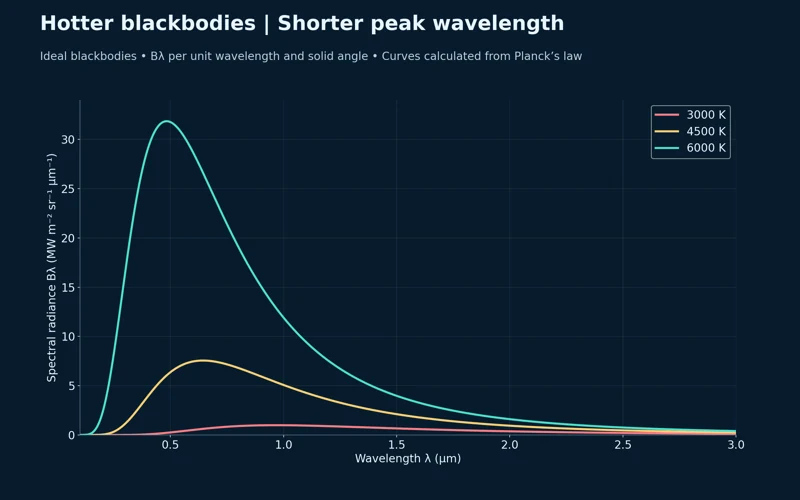 PHYSICS · 5 VISUALSBlackbody spectra and Wien’s lawConnect blackbody temperature with spectral shape, peak wavelength and total emission.
Hotter means a shorter peak wavelength
Three calculated spectra show a higher peak and shorter peak wavelength as temperature rises.
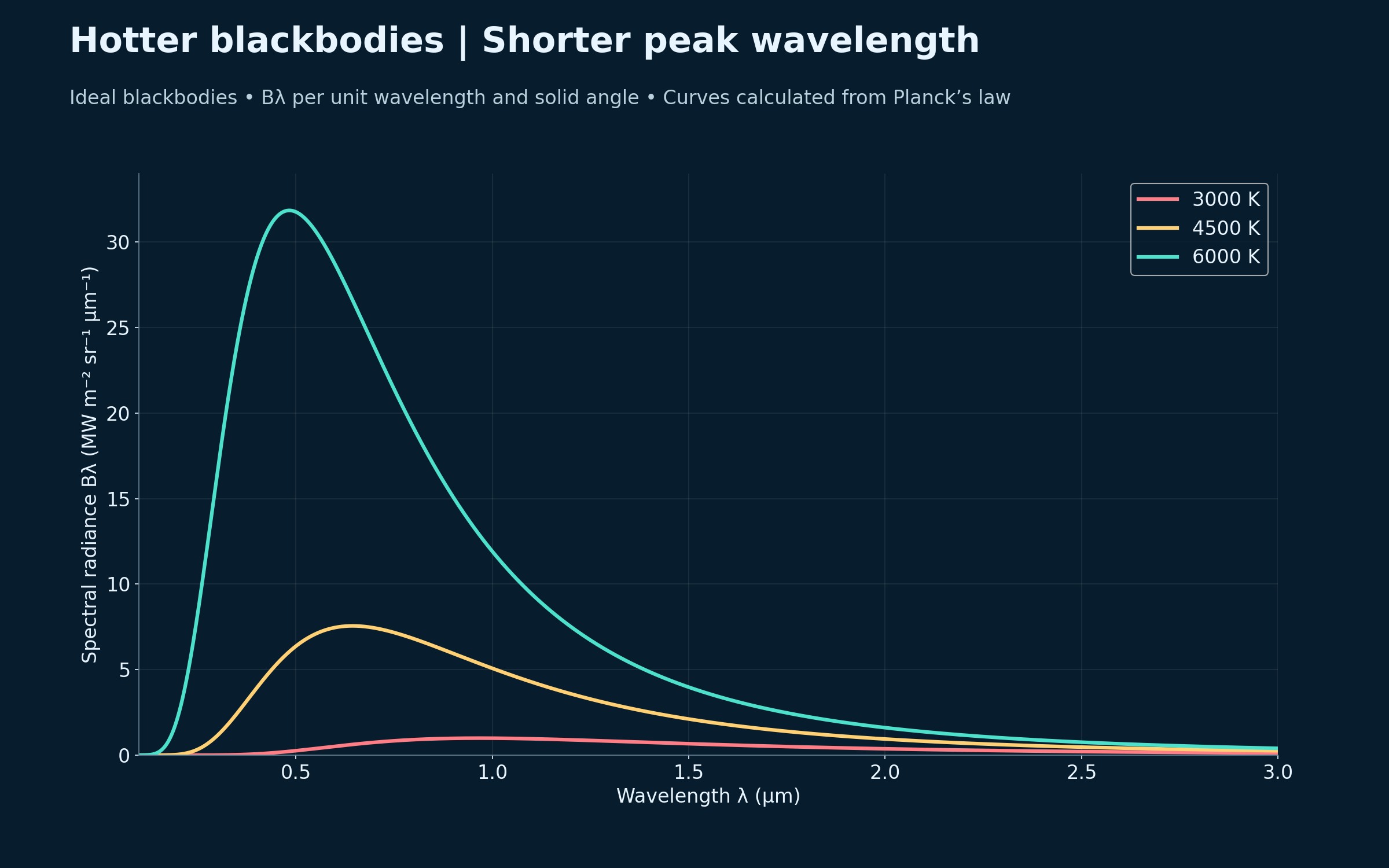

Three temperatures
Planck spectra mark approximate peaks of 0.966, 0.644 and 0.483 micrometres.
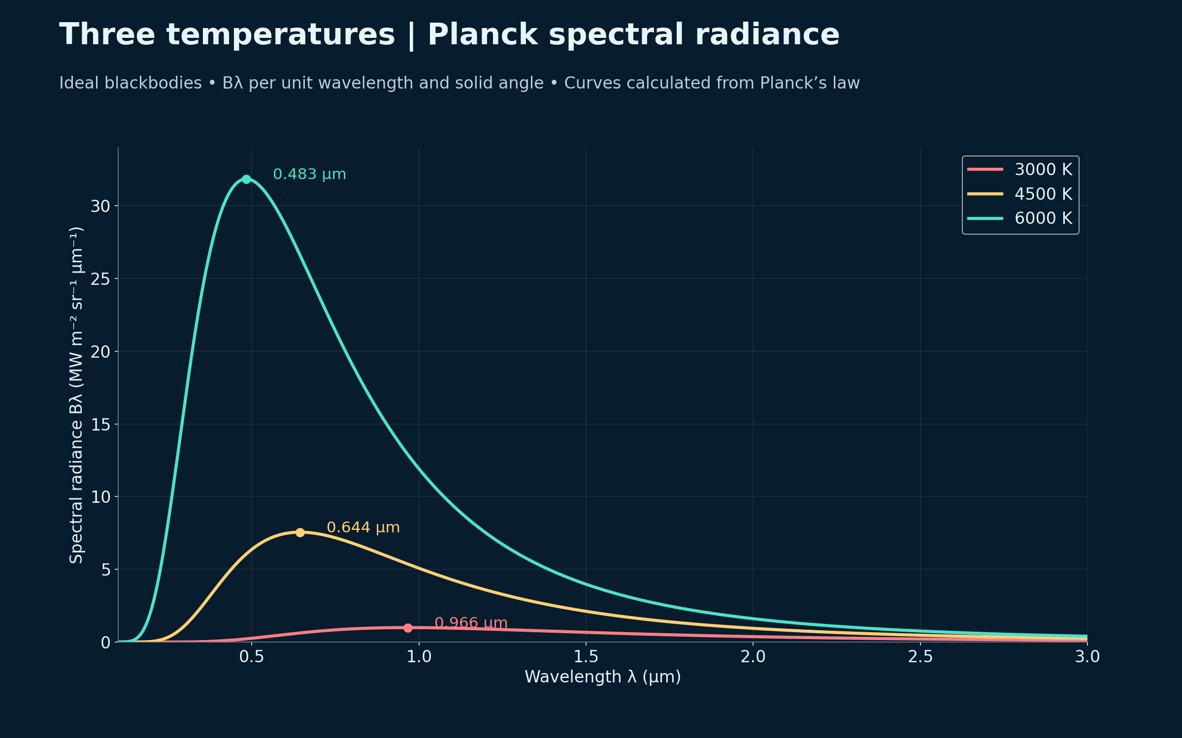
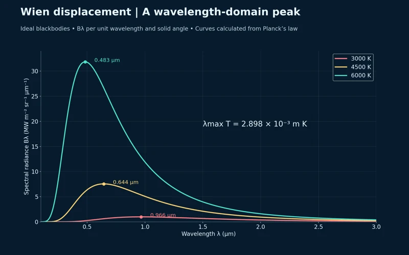
Wien displacement
The spectra accompany the wavelength-peak relation λmaxT = 2.898 × 10⁻³ m K.


The fourth-power law
An annotation explains that an ideal 6000 K blackbody emits sixteen times the flux per area of a 3000 K blackbody.

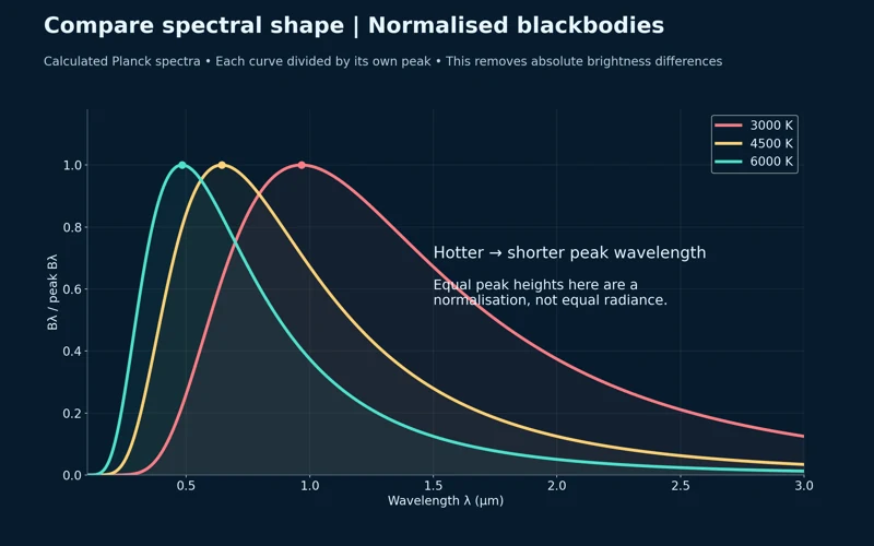
Comparing spectral shape
Peak-normalised curves compare shapes and peak positions without retaining absolute brightness differences.

Calculated Planck spectra for ideal blackbodies at 3000, 4500 and 6000 K. Spectral radiance is per wavelength and solid angle; total emitted flux is a separate quantity. These are not measured stellar spectra.
 PHYSICS · 5 VISUALSPhotoelectric effectSeparate the effects of frequency and intensity on photoelectron emission.
Light releases electrons
An apparatus illustration shows incident light releasing electrons from a metal surface toward a collector.


Frequency changes maximum kinetic energy
A linear graph begins at the threshold frequency and follows Kmax = hf − φ.


Intensity changes electron number
Dim and bright light at the same above-threshold frequency give the same maximum kinetic energy but different electron emission rates.


Stopping potential
A graph relates the stopping-potential magnitude to frequency through eVs = Kmax.


Three controlled tests
Below-threshold, above-threshold dim and above-threshold bright examples separate frequency from intensity.

Ideal one-photon photoelectric model with an example work function of 2.00 eV; multiphoton effects are excluded. Apparatus and ray colours are illustrative, not calibrated photographs.
 PHYSICS · 5 VISUALSAtomic emission and energy levelsConnect hydrogen energy-level gaps with absorbed and emitted photons.
A photon carries the difference
A hydrogen transition from n = 3 to n = 2 emits a photon of about 1.89 eV and 656 nm.
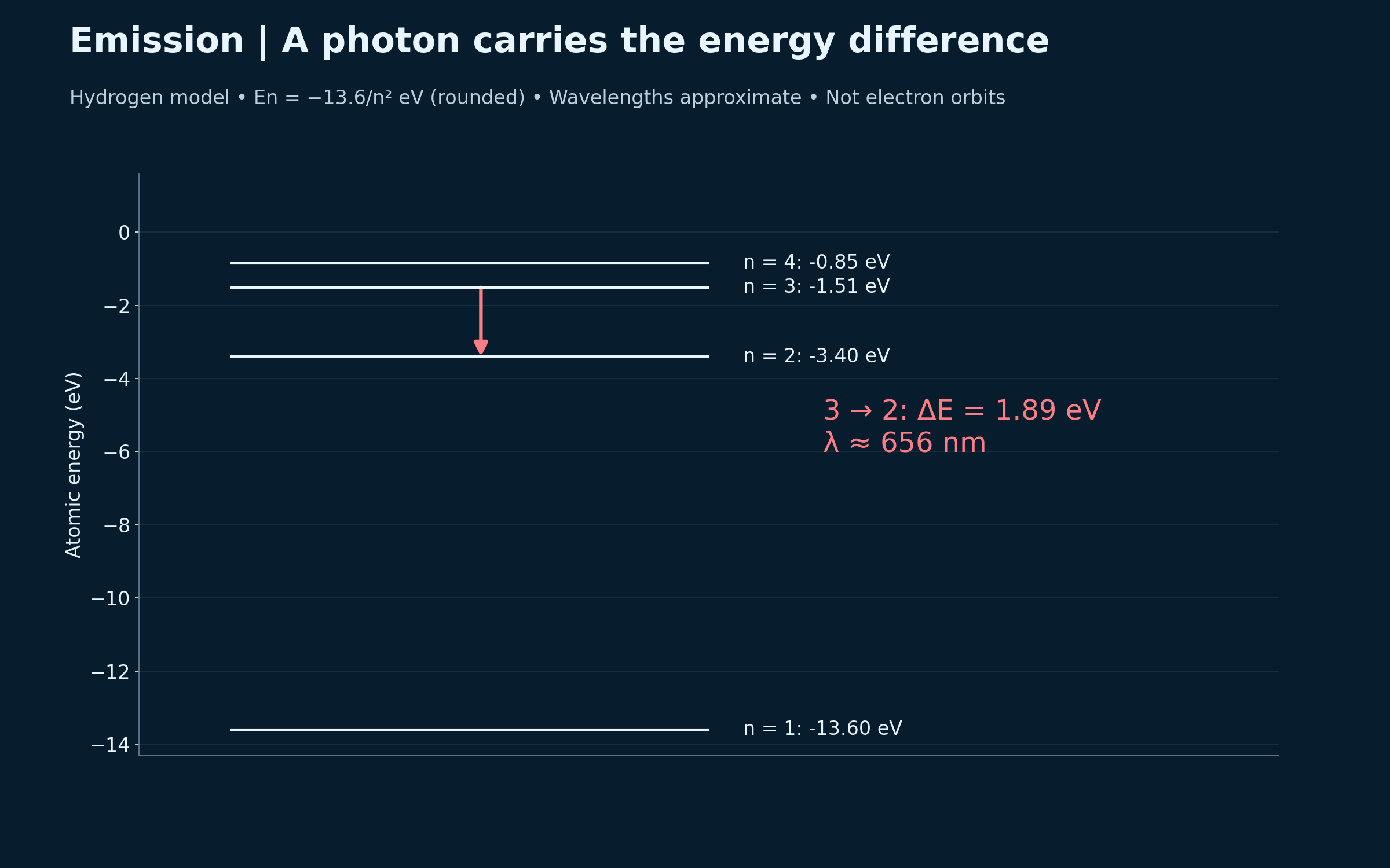

Absorption and emission
Opposite transitions between n = 1 and n = 2 show absorption and emission of the same energy gap.
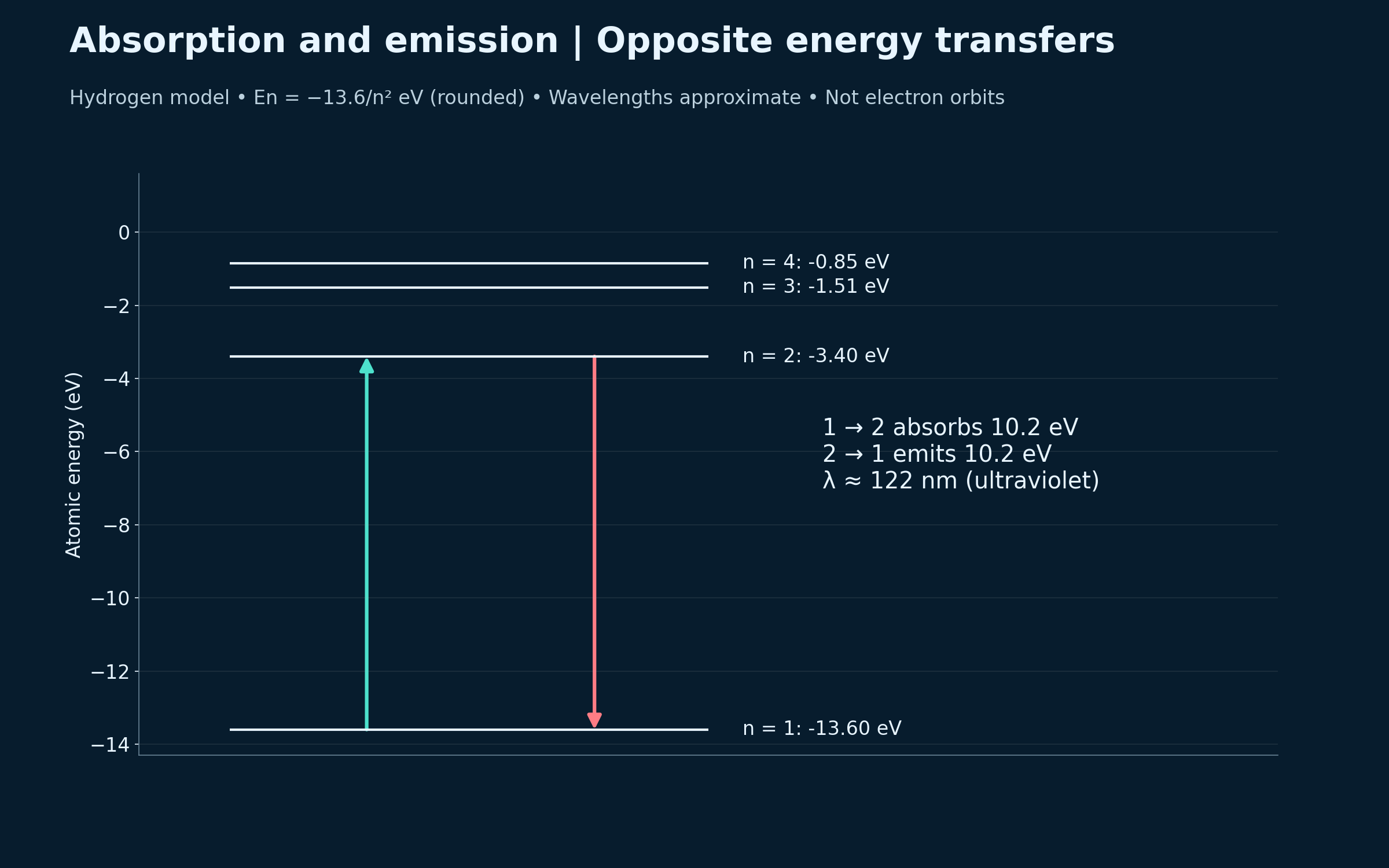
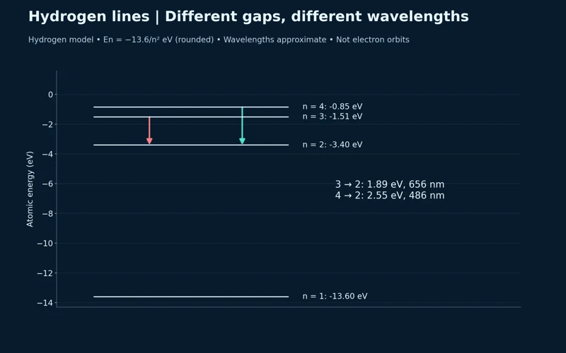
Different gaps, different wavelengths
Hydrogen transitions to n = 2 compare approximately 656 nm and 486 nm photons.


Calculating the Balmer H-alpha photon
The n = 3 to n = 2 gap is converted to wavelength using ΔE = hf = hc/λ.


Line positions follow wavelength
A simplified Balmer spectrum marks lines near 410, 434, 486 and 656 nm.

Rounded hydrogen energy levels from En = −13.6/n² eV. Wavelengths are approximate; level lines are energies, not electron orbits. Spectrum-line heights are arbitrary and do not predict intensity.
 PHYSICS · 5 VISUALSAlpha, beta and gamma penetrationCompare radiation types and explain why shielding attenuates gamma radiation rather than eliminating it exactly.
Comparing ionising radiation
Alpha, beta-minus and gamma paths are compared with paper, aluminium and dense shielding.


Different particles, different penetration
The diagram identifies alpha as a helium nucleus, beta-minus as an electron and gamma as an uncharged photon.


Gamma rays are attenuated
An exponential curve shows transmitted uncollided gamma intensity decreasing with shield thickness.


Half-value layers
The attenuation curve marks successive reductions to 50, 25, 12.5 and 6.25 percent.
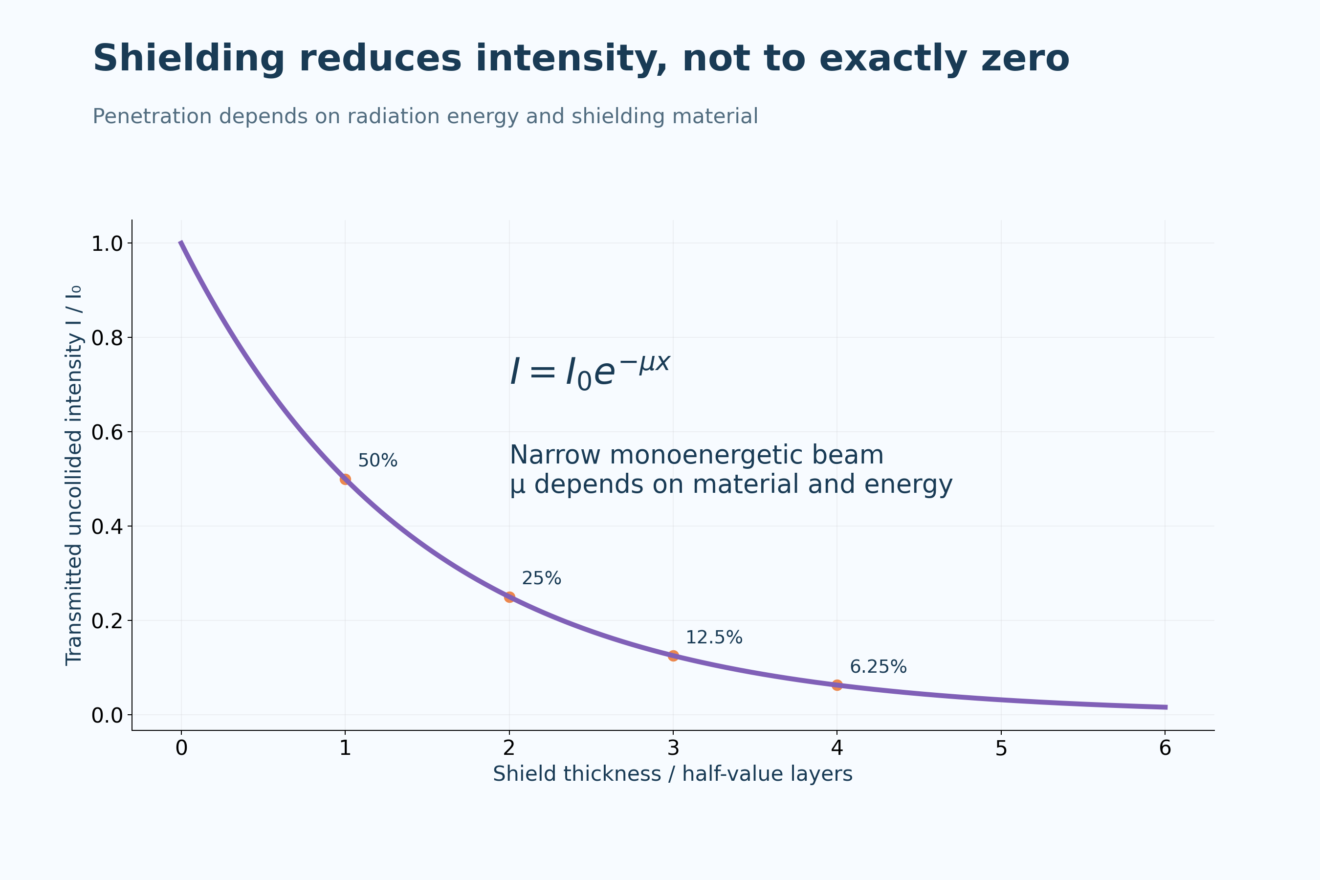

External and internal exposure differ
The comparison notes that alpha radiation is weakly penetrating externally but can be hazardous inside the body.

Qualitative penetration comparisons depend on radiation energy and shielding material. Gamma plots model uncollided intensity in a narrow monoenergetic beam; they are not universal shielding specifications.
 PHYSICS · 5 VISUALSNuclear fissionFollow one possible uranium-235 fission channel and check conservation before considering successive events.
Neutron-induced fission
A uranium-235 example produces barium-141, krypton-92 and three neutrons.
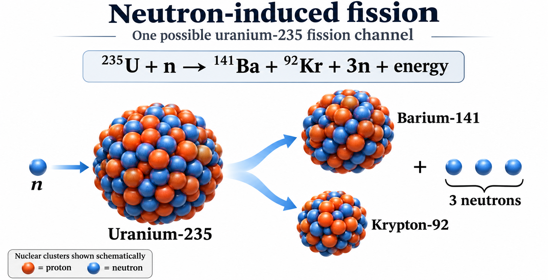
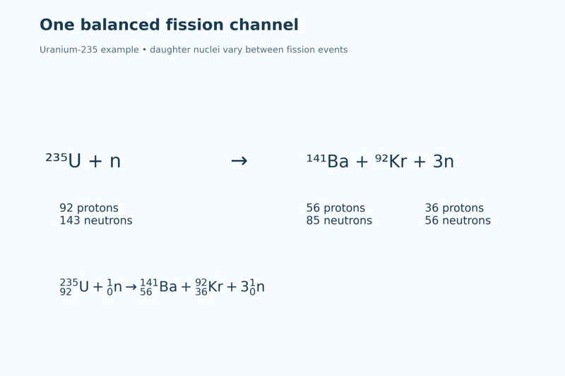
One balanced channel
Nuclide notation and proton-neutron counts identify the reactant and example daughter nuclei.


Mass number and charge are conserved
The equation checks 235 + 1 = 141 + 92 + 3 and 92 = 56 + 36.


Successive generations
A schematic chain shows one successor fission per event while other neutrons escape or are captured without fission.


Steady and increasing populations
Two branching diagrams compare one event per generation with a doubling sequence.

One selected uranium-235 fission channel, not the only possible products. Large nuclear clusters and chain diagrams are schematic rather than measured nuclear shapes or a reactor design.
 PHYSICS · 5 VISUALSNuclear fusionUse deuterium–tritium fusion to connect nucleon conservation with released energy.
Deuterium–tritium fusion
Two light nuclei combine to produce helium-4 and a neutron, with less total product rest mass.


Five nucleons before and after
The particle model retains two protons and three neutrons through the reaction.
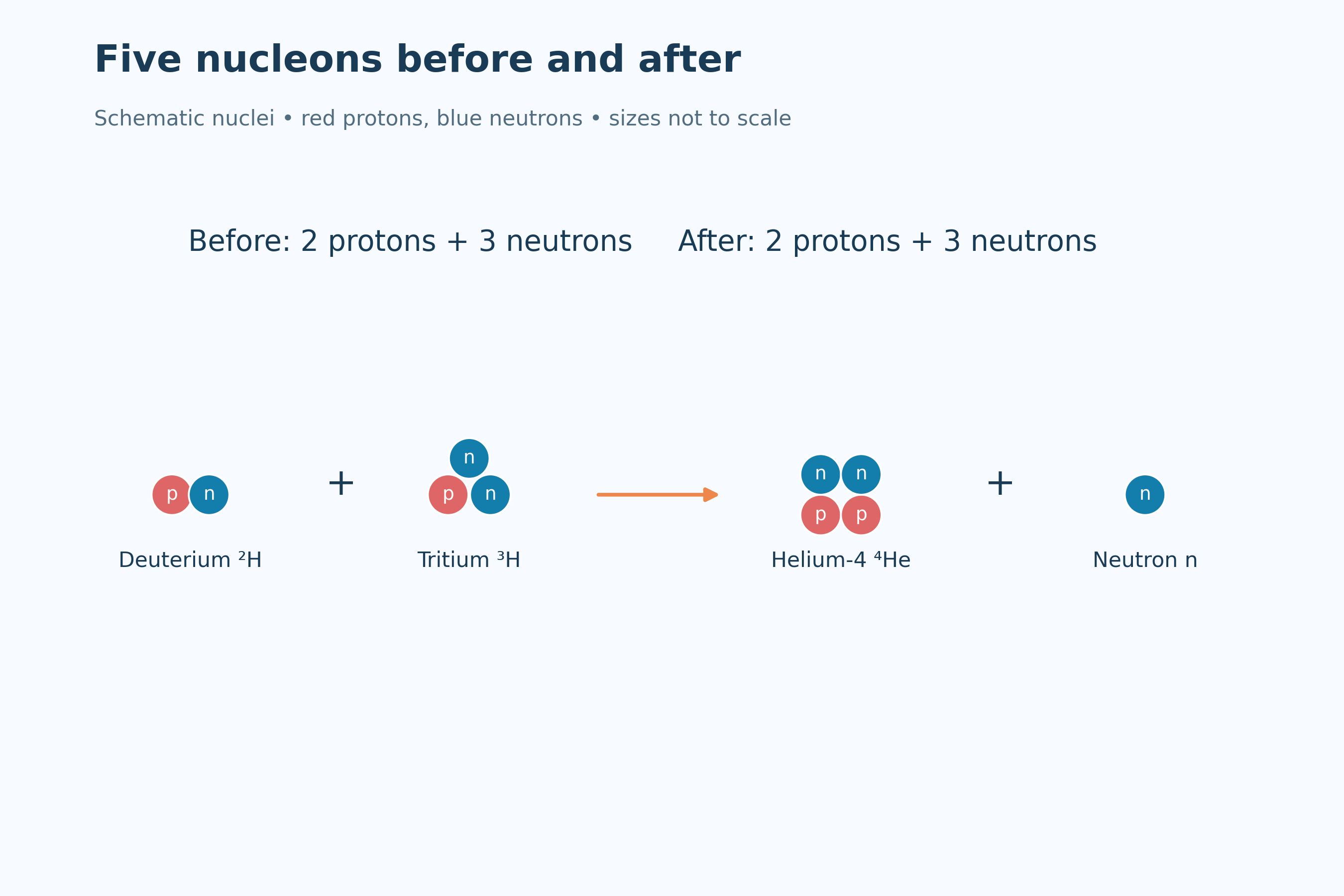

Energy released
The model connects a mass difference with approximately 17.6 MeV of released energy.
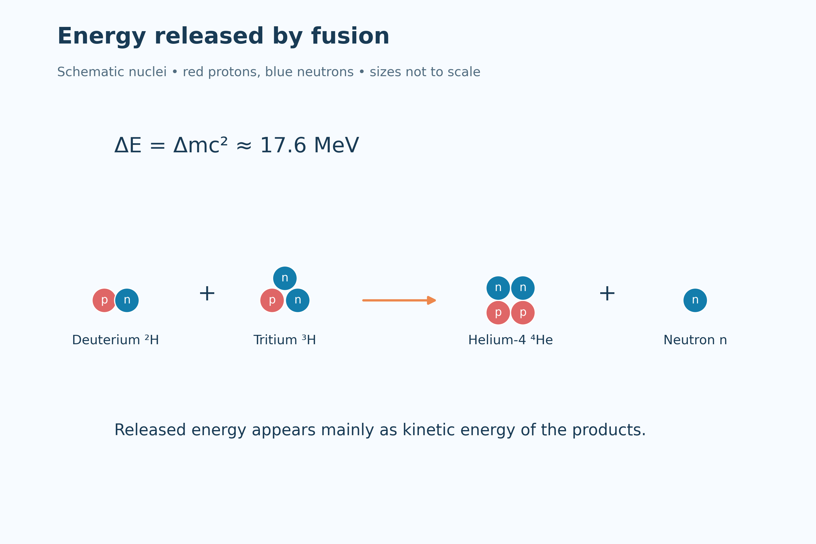

Conserving mass number and charge
Nuclide notation checks mass numbers 2 + 3 = 4 + 1 and charge numbers 1 + 1 = 2 + 0.


Energy partition
A schematic allocates about 3.5 MeV to helium-4 and 14.1 MeV to the neutron.

Schematic deuterium–tritium nuclei, not measured shapes. The approximately 3.5 MeV and 14.1 MeV product energies assume initially slow reactants.
 PHYSICS · 5 VISUALSGravitational fields and orbital motionExplain a circular orbit as continuous free fall and connect radius with speed and energy.
Continuous free fall
A circular-orbit diagram distinguishes tangential velocity from inward gravitational acceleration.


Gravity points towards the planet
Four orbital positions show inward gravity and changing tangential velocity direction.


An orbit at radius r
The diagram relates field strength and orbital speed to distance measured from the planet’s centre.


Comparing two circular orbits
Doubling orbital radius gives one-quarter of the gravitational field strength and 1/√2 of the orbital speed.


A bound circular orbit
A satellite illustration lists kinetic, gravitational potential and total orbital energy with potential zero at infinity.
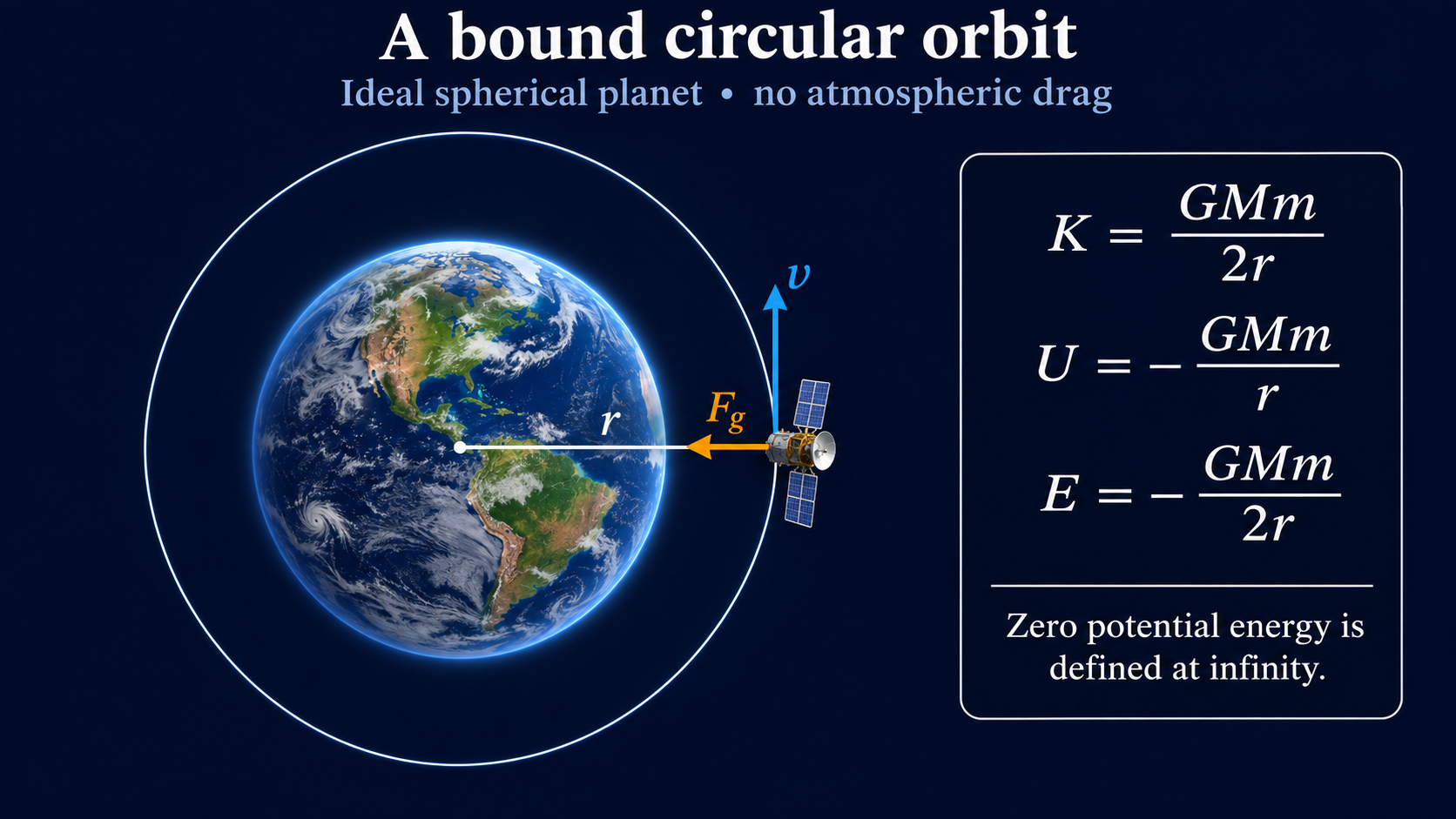
Newtonian circular-orbit models around an ideal spherical planet with no atmospheric drag. Direction arrows are not magnitude comparisons unless stated; the satellite illustration is not a measured orbit.
 PHYSICS · 5 VISUALSThe Hertzsprung–Russell diagramRead stellar luminosity and temperature together, then connect them with radius and evolution.
The main stellar regions
A schematic H–R diagram locates the main sequence, giants, white dwarfs and the Sun.


Temperature decreases to the right
Spectral classes O through M accompany the reversed surface-temperature axis.

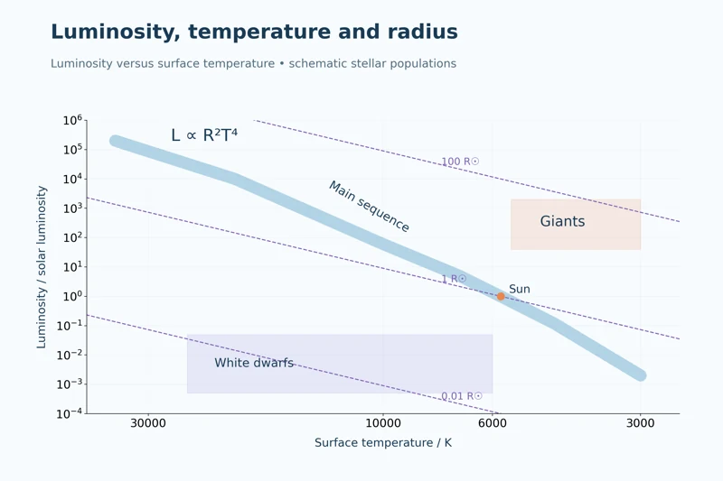
Luminosity, temperature and radius
Constant-radius guide lines connect stellar position with the proportionality L ∝ R²T⁴.
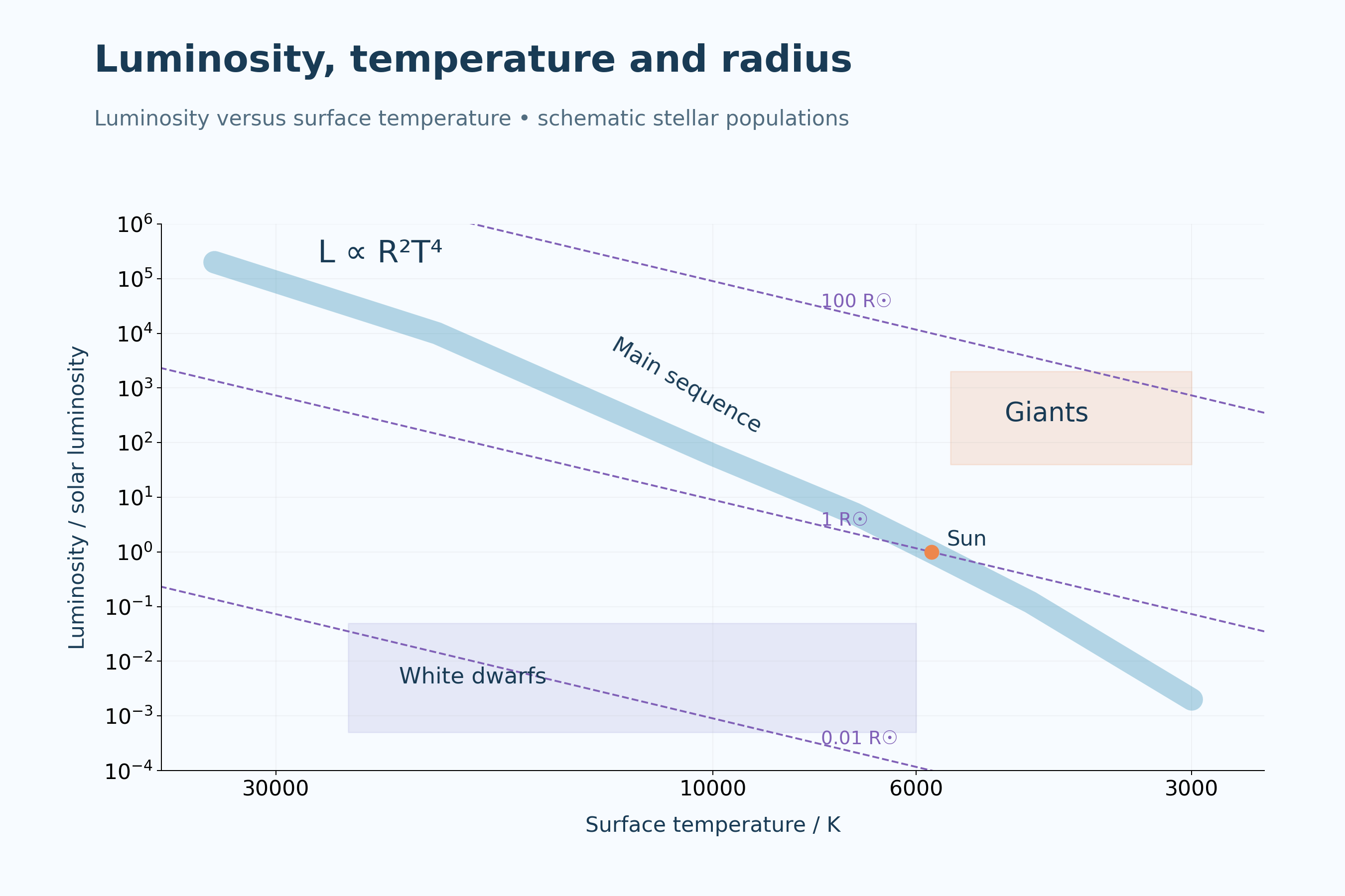

Same temperature, different radii
Two stars at 5800 K compare a tenfold radius increase with a hundredfold luminosity increase.
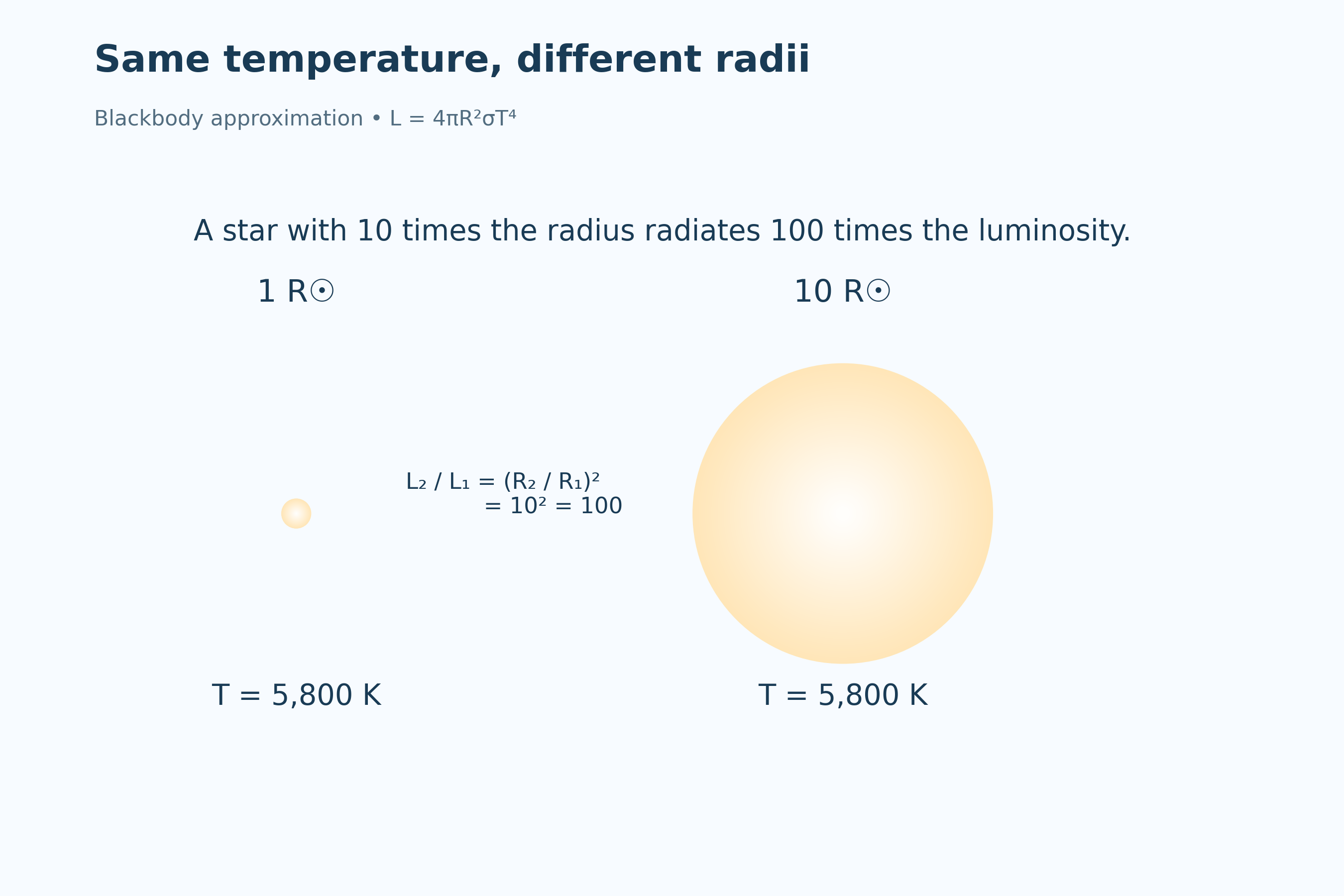
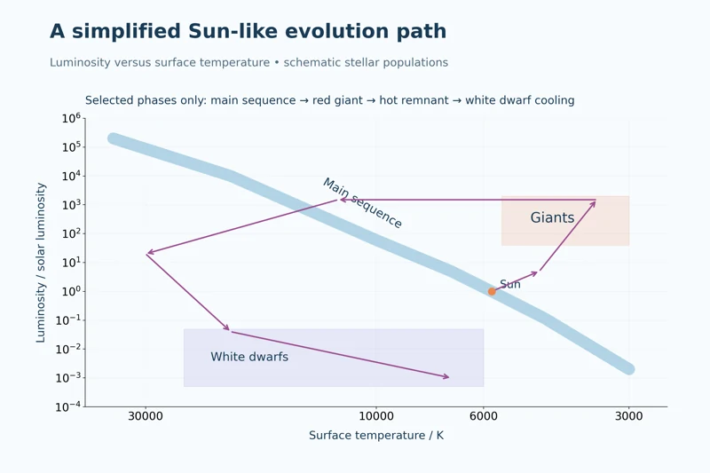
A simplified Sun-like evolution path
A selected-phase track links the main sequence, red giant, hot remnant and cooling white dwarf stages.
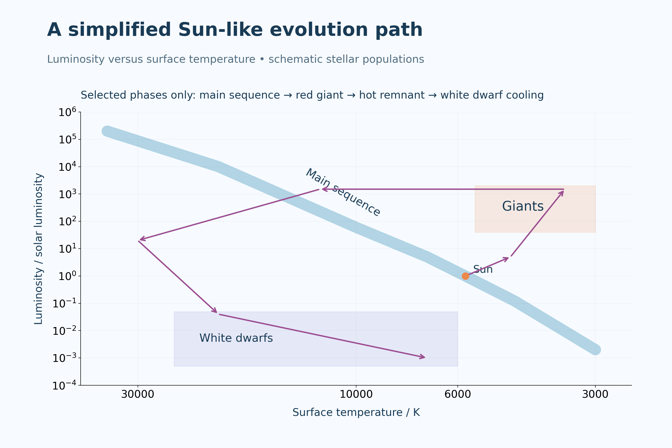
Schematic stellar populations on logarithmic axes, not a measured catalogue. Radius comparisons use a blackbody approximation; the Sun-like evolution path shows selected phases only and is not to evolutionary timescale.
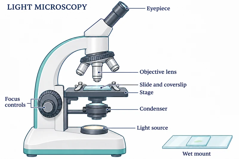 BIOLOGY · B01 · 3 VISUALSLight microscopy and wet mountsObserve prepared cells and tissues using a light microscope and wet-mount slide.
Labelled schematic
Observe prepared cells and tissues using a light microscope and wet-mount slide.
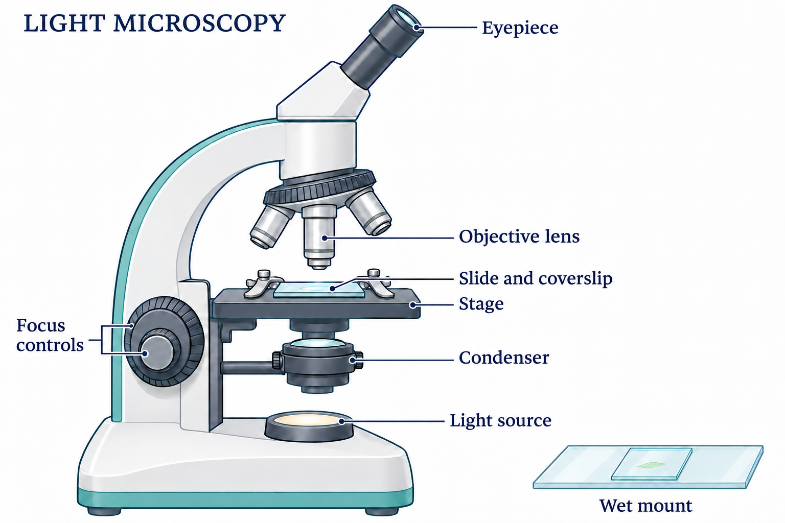

Realistic apparatus view
Observe prepared cells and tissues using a light microscope and wet-mount slide.
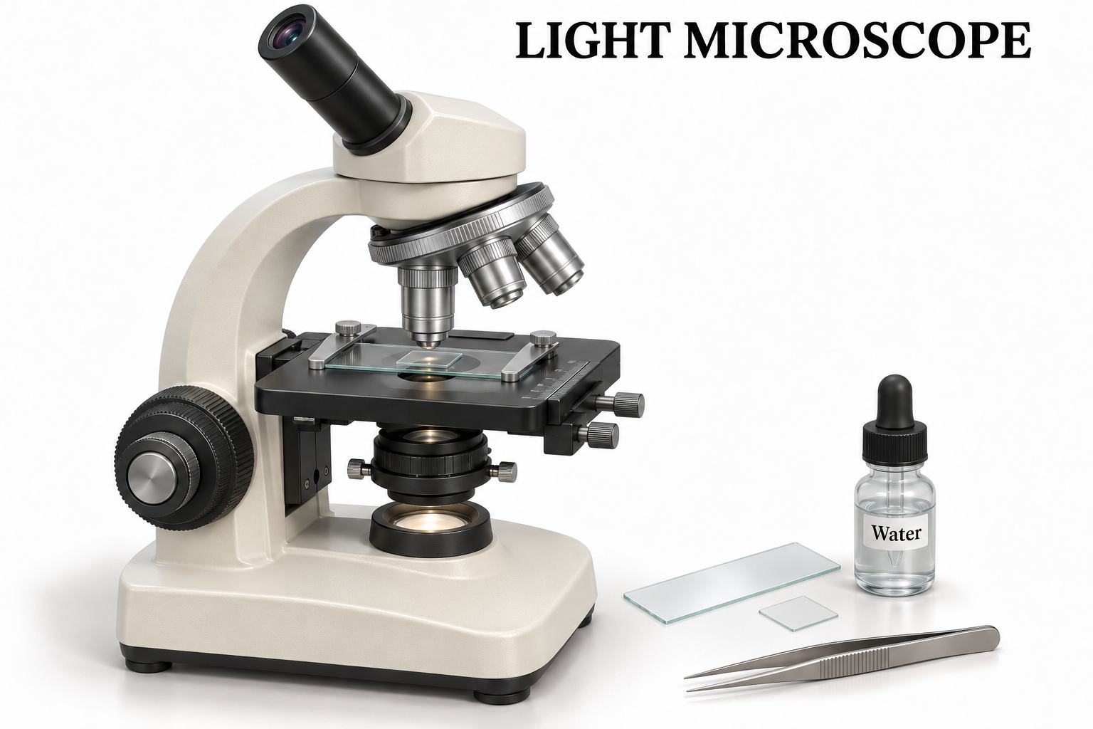

Critical detail
Observe prepared cells and tissues using a light microscope and wet-mount slide.

The enlarged coverslip section explains assembly; it is not to scale.
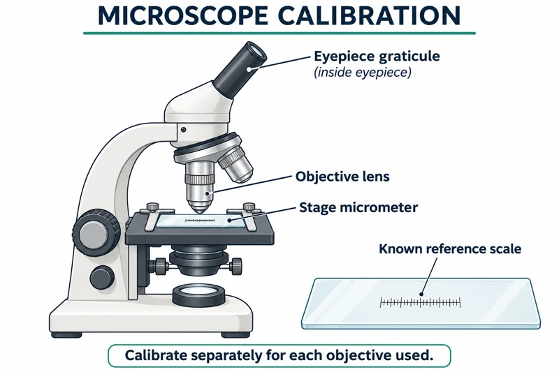 BIOLOGY · B02 · 3 VISUALSMicroscope calibrationCompare an eyepiece graticule with a stage micrometer to establish a specimen measurement scale.
Labelled schematic
Compare an eyepiece graticule with a stage micrometer to establish a specimen measurement scale.


Realistic apparatus view
Compare an eyepiece graticule with a stage micrometer to establish a specimen measurement scale.
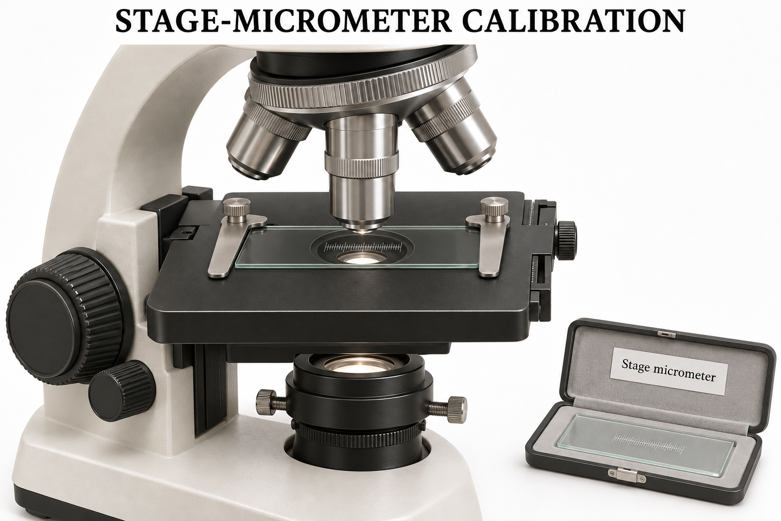
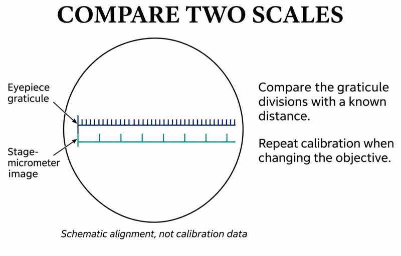
Critical detail
Compare an eyepiece graticule with a stage micrometer to establish a specimen measurement scale.
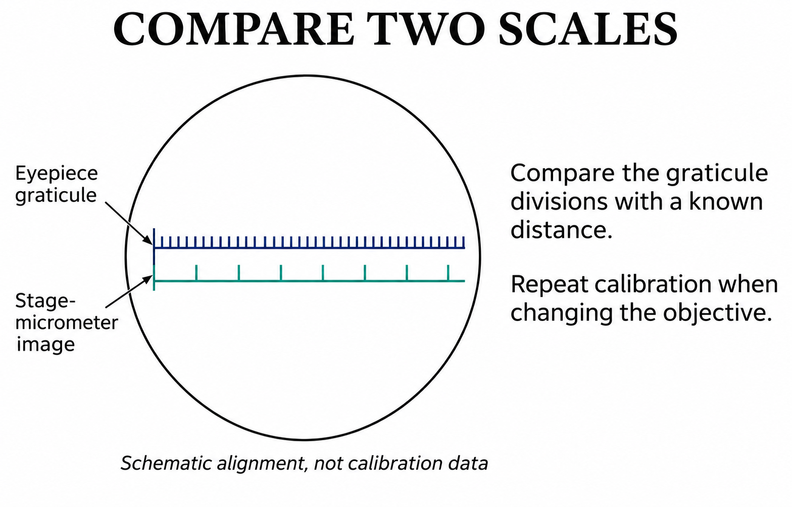
The illustrated scale comparison is conceptual and must not be used to calculate a calibration.
 BIOLOGY · B03 · 3 VISUALSRoot-tip squash preparationShow how a thin root-tip squash is arranged for microscopy of dividing cells.
Labelled schematic
Show how a thin root-tip squash is arranged for microscopy of dividing cells.
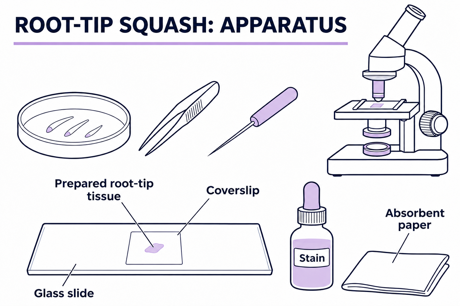

Realistic apparatus view
Show how a thin root-tip squash is arranged for microscopy of dividing cells.

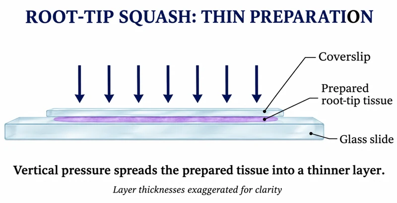
Critical detail
Show how a thin root-tip squash is arranged for microscopy of dividing cells.

The images show the prepared-tissue principle, not the complete tissue-treatment procedure.
 BIOLOGY · B04 · 3 VISUALSOsmosis in plant tissueCompare changes in plant-tissue mass after exposure to different solution concentrations.
Labelled schematic
Compare changes in plant-tissue mass after exposure to different solution concentrations.


Realistic apparatus view
Compare changes in plant-tissue mass after exposure to different solution concentrations.

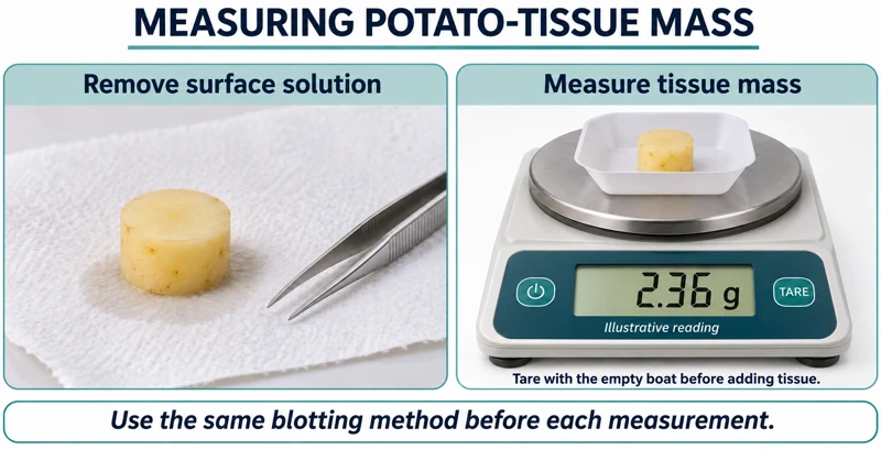
Critical detail
Compare changes in plant-tissue mass after exposure to different solution concentrations.

Displayed masses are illustrative; consistent blotting and a tared weighing vessel matter.
 BIOLOGY · B05 · 3 VISUALSDialysis-tubing membrane modelUse dialysis tubing to investigate movement of substances across a selectively permeable barrier.
Labelled schematic
Use dialysis tubing to investigate movement of substances across a selectively permeable barrier.


Realistic apparatus view
Use dialysis tubing to investigate movement of substances across a selectively permeable barrier.
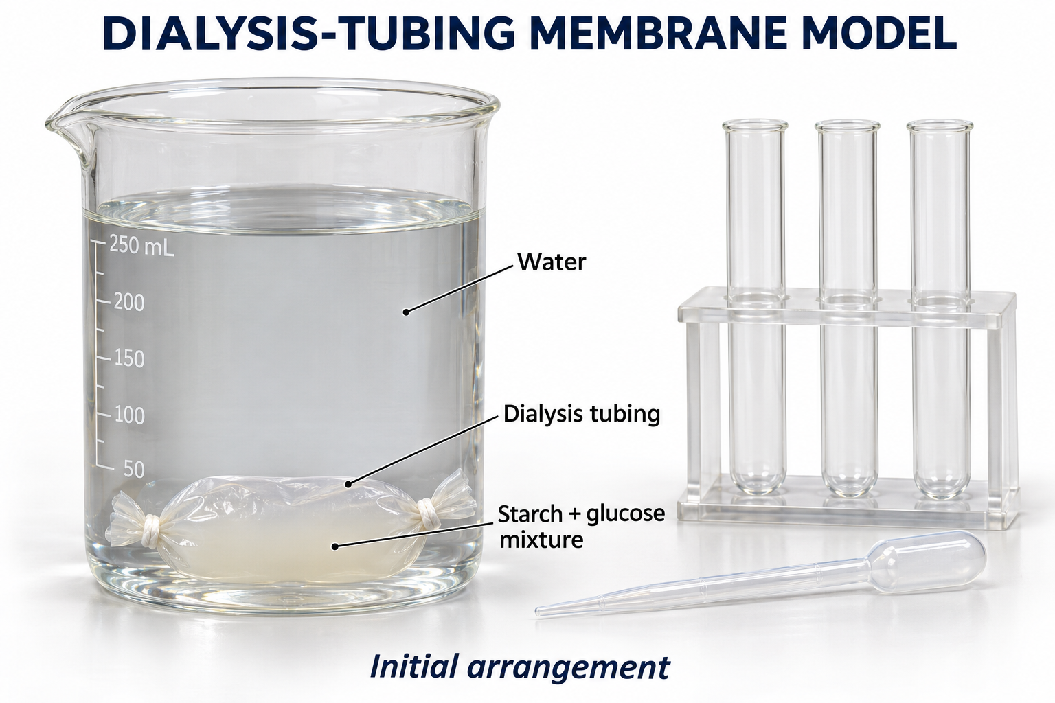

Critical detail
Use dialysis tubing to investigate movement of substances across a selectively permeable barrier.
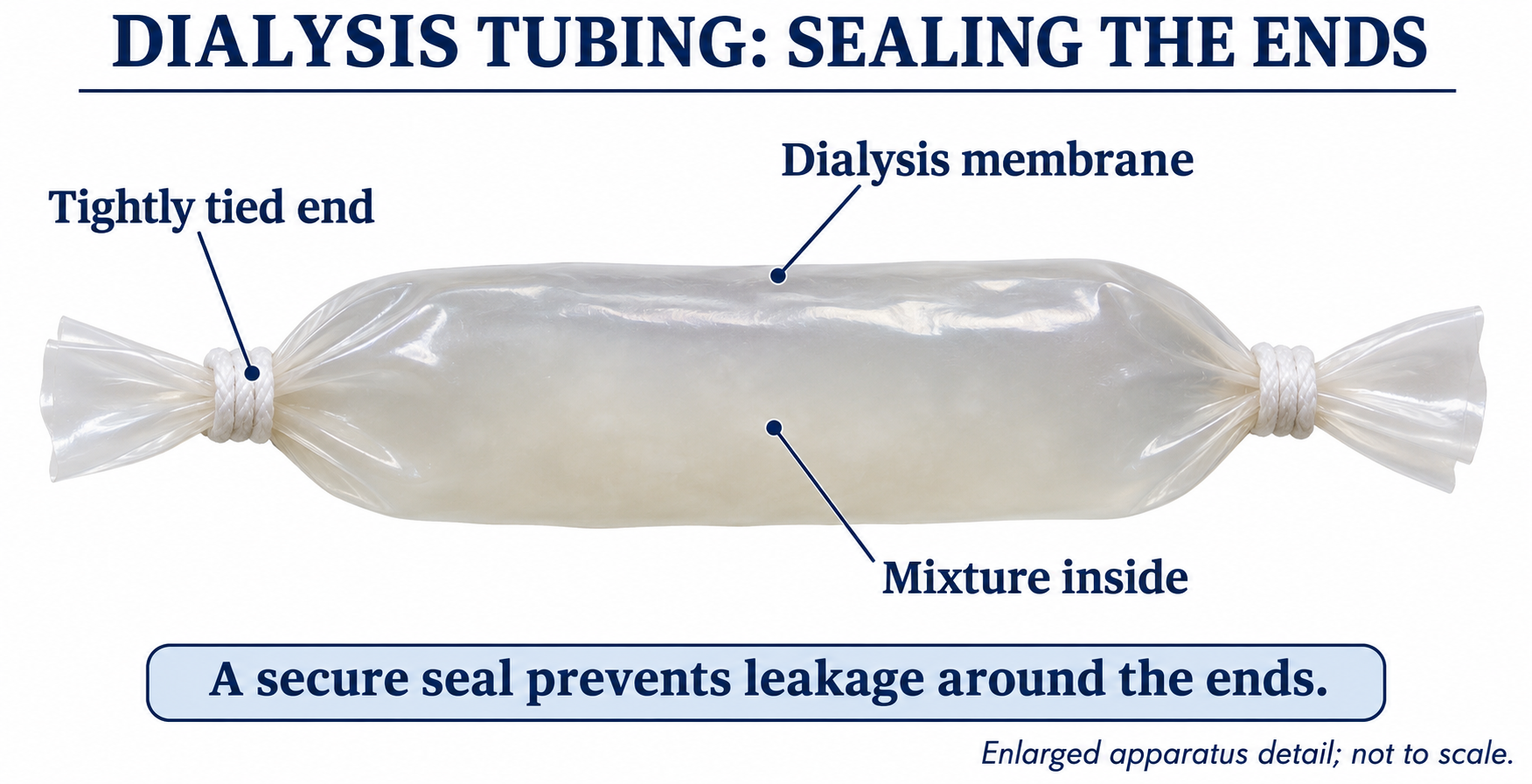
The equipment overview does not show every inside-and-outside test needed to interpret a result.
 BIOLOGY · B06 · 3 VISUALSDiffusion through agar blocksCompare diffusion into agar blocks of different sizes.
Labelled schematic
Compare diffusion into agar blocks of different sizes.


Realistic apparatus view
Compare diffusion into agar blocks of different sizes.
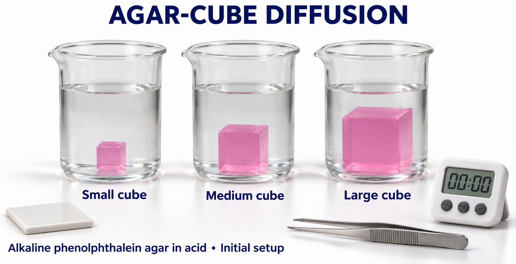

Critical detail
Compare diffusion into agar blocks of different sizes.

Colour boundaries and ruler marks illustrate the principle rather than measured diffusion depths.
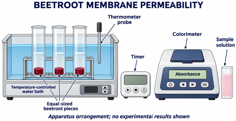 BIOLOGY · B07 · 3 VISUALSBeetroot membrane permeabilityMeasure pigment leakage from beetroot samples using controlled temperature treatments and colorimetry.
Labelled schematic
Measure pigment leakage from beetroot samples using controlled temperature treatments and colorimetry.


Realistic apparatus view
Measure pigment leakage from beetroot samples using controlled temperature treatments and colorimetry.


Critical detail
Measure pigment leakage from beetroot samples using controlled temperature treatments and colorimetry.

Tubes sharing one bath experience the same temperature; remove tissue before optical measurement.
 BIOLOGY · B08 · 3 VISUALSPlasmolysis slide setupExchange solutions beneath a coverslip to investigate plasmolysis in plant cells.
Labelled schematic
Exchange solutions beneath a coverslip to investigate plasmolysis in plant cells.


Realistic apparatus view
Exchange solutions beneath a coverslip to investigate plasmolysis in plant cells.


Critical detail
Exchange solutions beneath a coverslip to investigate plasmolysis in plant cells.

The images show solution exchange, not observed cellular results.
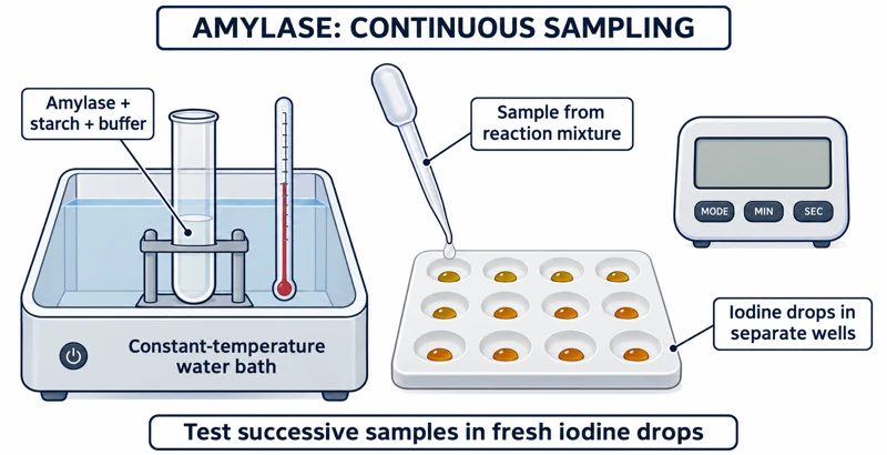 BIOLOGY · B09 · 3 VISUALSAmylase and starch samplingFollow starch breakdown by transferring timed reaction samples to iodine wells.
Labelled schematic
Follow starch breakdown by transferring timed reaction samples to iodine wells.
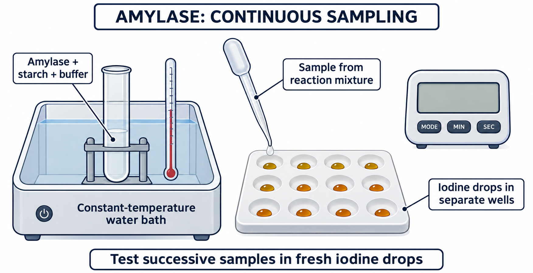

Realistic apparatus view
Follow starch breakdown by transferring timed reaction samples to iodine wells.
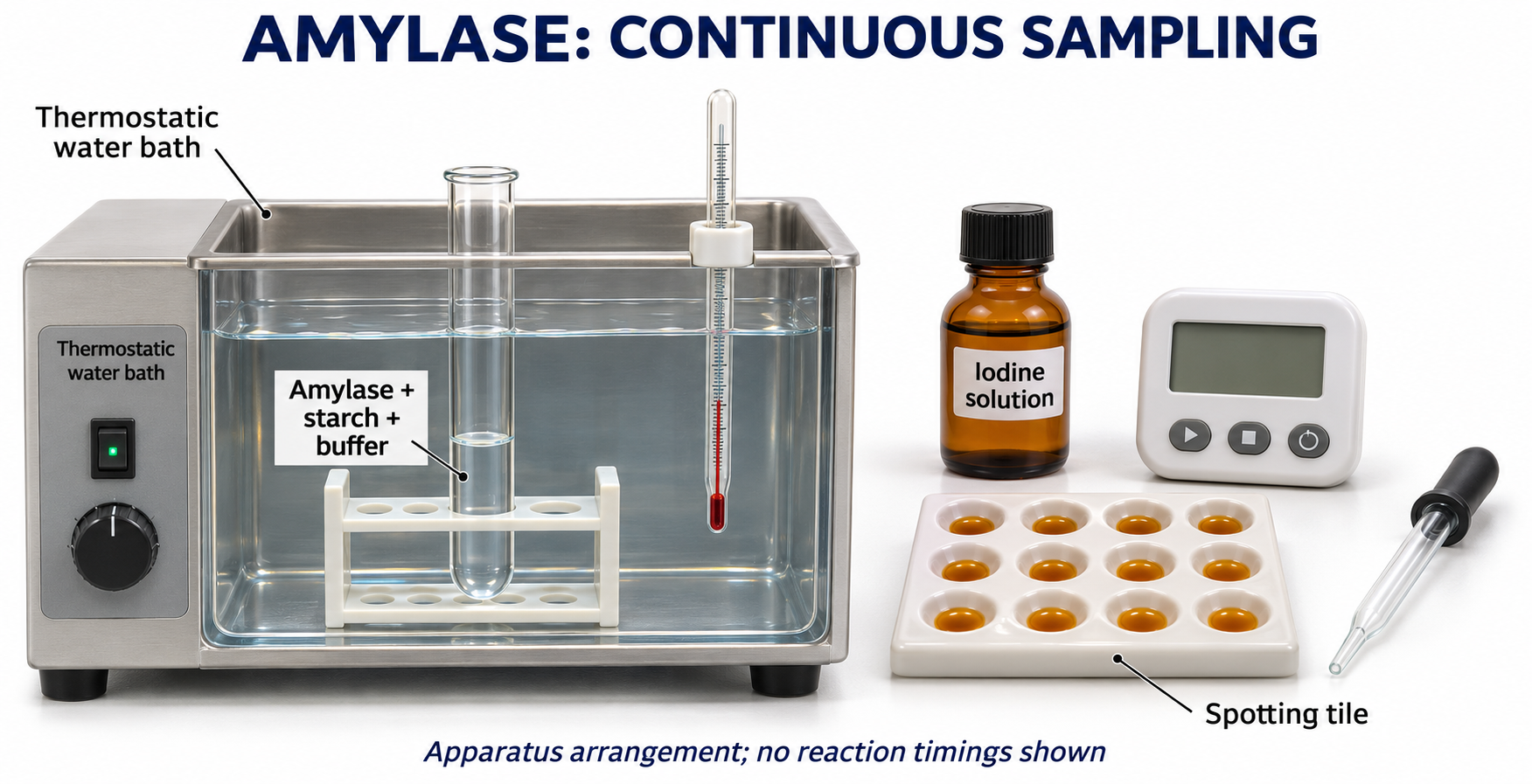

Critical detail
Follow starch breakdown by transferring timed reaction samples to iodine wells.

The test colours illustrate possible observations, not a measured time series.
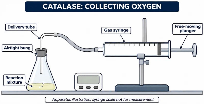 BIOLOGY · B10 · 3 VISUALSCatalase with a gas syringeFollow oxygen production during a catalase reaction by collecting gas in a syringe.
Labelled schematic
Follow oxygen production during a catalase reaction by collecting gas in a syringe.


Realistic apparatus view
Follow oxygen production during a catalase reaction by collecting gas in a syringe.


Critical detail
Follow oxygen production during a catalase reaction by collecting gas in a syringe.

Initial trapped air means the collected gas is not necessarily pure oxygen.
 BIOLOGY · B11 · 3 VISUALSTrypsin and milk colorimetryFollow changes in milk turbidity during a trypsin reaction using a colorimeter.
Labelled schematic
Follow changes in milk turbidity during a trypsin reaction using a colorimeter.

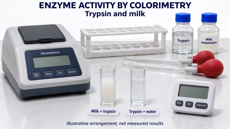
Realistic apparatus view
Follow changes in milk turbidity during a trypsin reaction using a colorimeter.

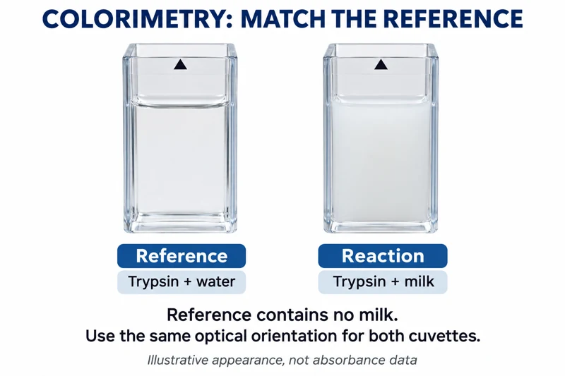
Critical detail
Follow changes in milk turbidity during a trypsin reaction using a colorimeter.
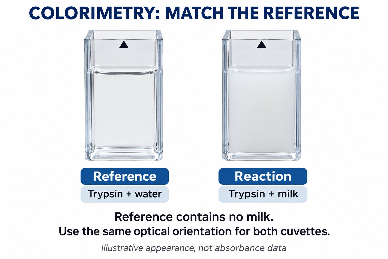
The trypsin-and-water reference differs from the trypsin-and-milk reaction; this is not a colour-matching endpoint.
 BIOLOGY · B12 · 3 VISUALSFood-test apparatusArrange test tubes, reagents and a water bath for qualitative biological-molecule tests.
Labelled schematic
Arrange test tubes, reagents and a water bath for qualitative biological-molecule tests.


Realistic apparatus view
Arrange test tubes, reagents and a water bath for qualitative biological-molecule tests.

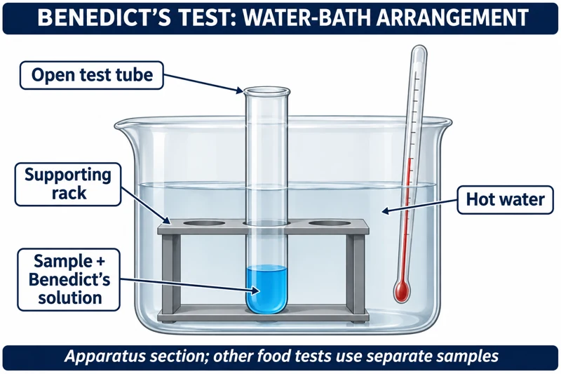
Critical detail
Arrange test tubes, reagents and a water bath for qualitative biological-molecule tests.
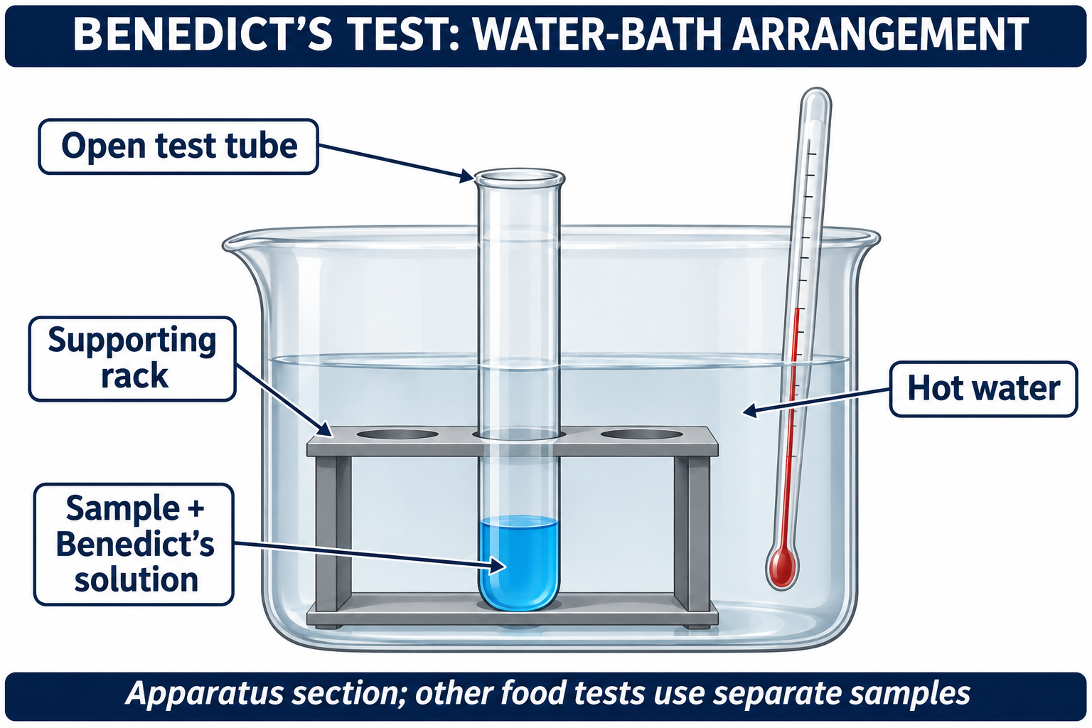
The images show the starting apparatus without claiming test outcomes.
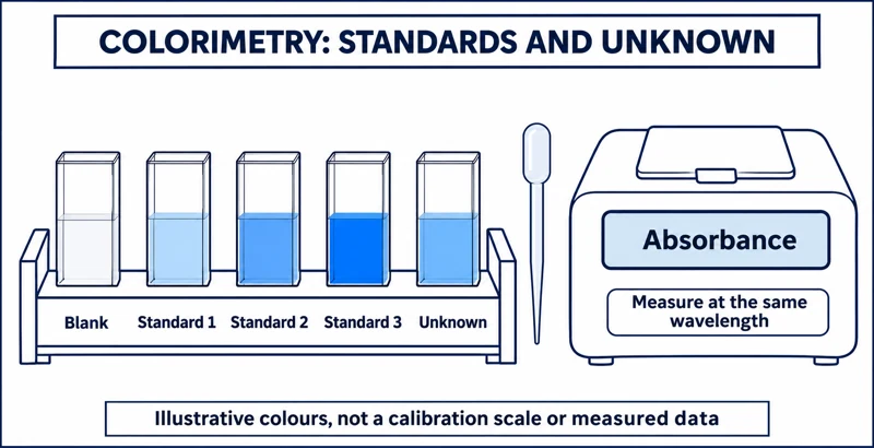 BIOLOGY · B13 · 3 VISUALSColorimetric concentration standardsUse a series of standards and a colorimeter to estimate an unknown concentration.
Labelled schematic
Use a series of standards and a colorimeter to estimate an unknown concentration.


Realistic apparatus view
Use a series of standards and a colorimeter to estimate an unknown concentration.
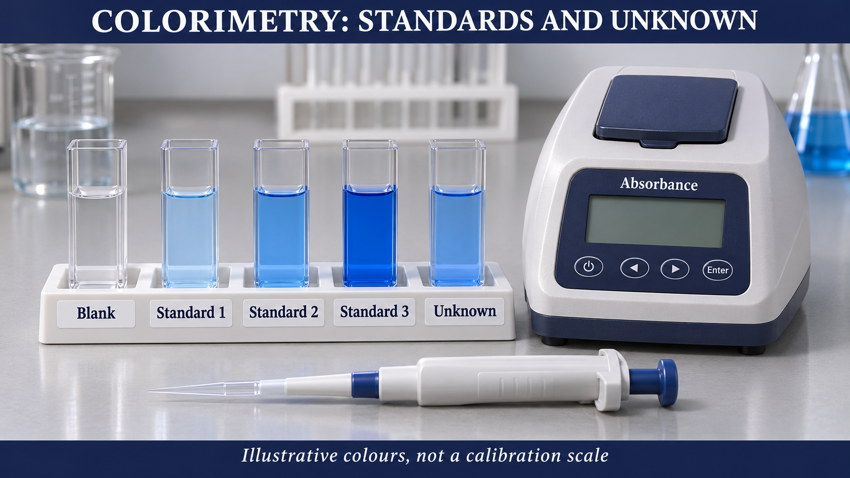
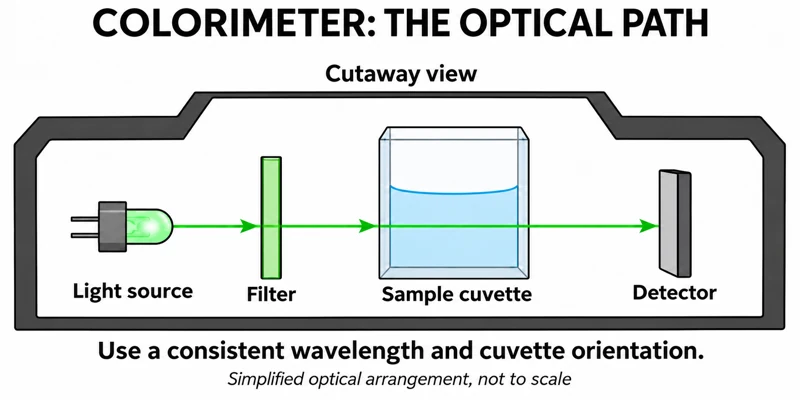
Critical detail
Use a series of standards and a colorimeter to estimate an unknown concentration.

Colours and optics are illustrative; a suitable wavelength depends on the actual assay.
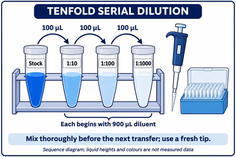 BIOLOGY · B14 · 3 VISUALSTenfold serial dilutionPrepare a sequence of tenfold dilutions using accurate pipetting and mixing.
Labelled schematic
Prepare a sequence of tenfold dilutions using accurate pipetting and mixing.


Realistic apparatus view
Prepare a sequence of tenfold dilutions using accurate pipetting and mixing.

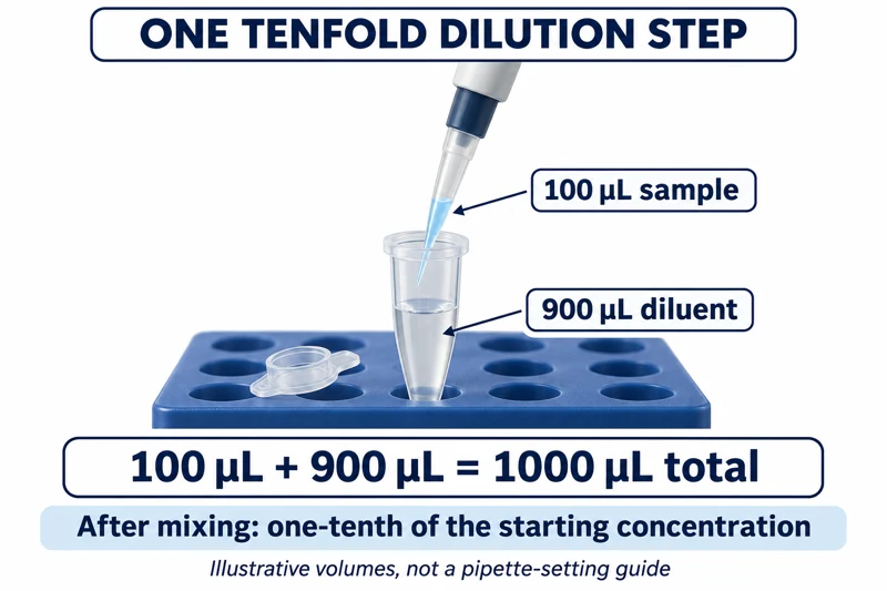
Critical detail
Prepare a sequence of tenfold dilutions using accurate pipetting and mixing.
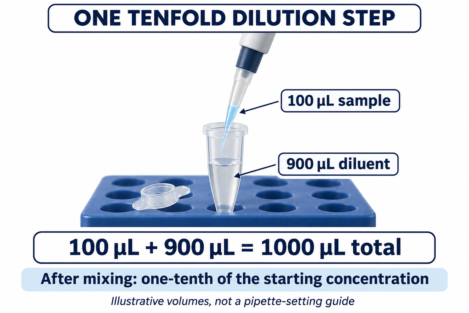
Each step represents 100 microlitres transferred into 900 microlitres; liquid heights are not measurement data.
 BIOLOGY · B15 · 3 VISUALSPondweed gas collectionCollect gas from illuminated aquatic plant material to investigate photosynthesis.
Labelled schematic
Collect gas from illuminated aquatic plant material to investigate photosynthesis.
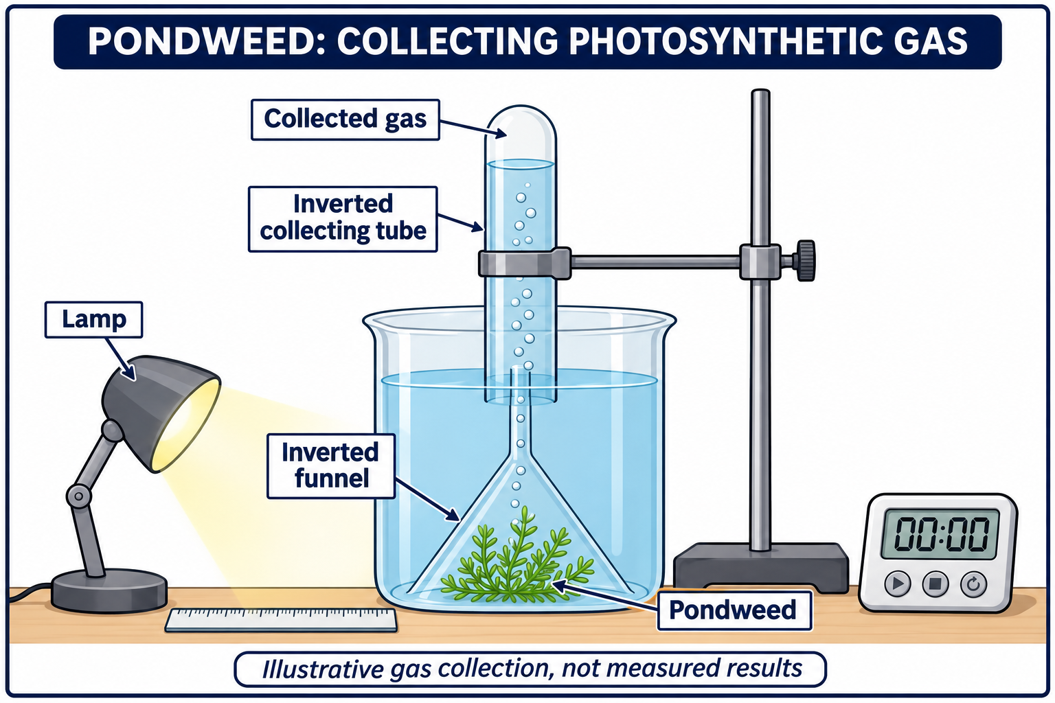

Realistic apparatus view
Collect gas from illuminated aquatic plant material to investigate photosynthesis.
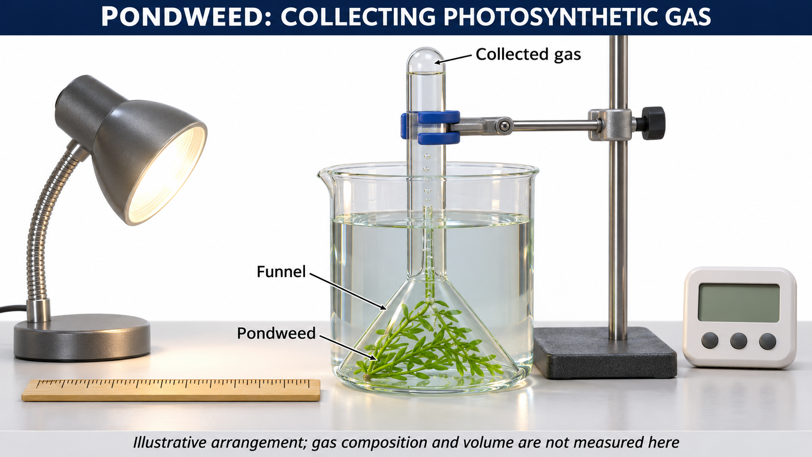

Critical detail
Collect gas from illuminated aquatic plant material to investigate photosynthesis.
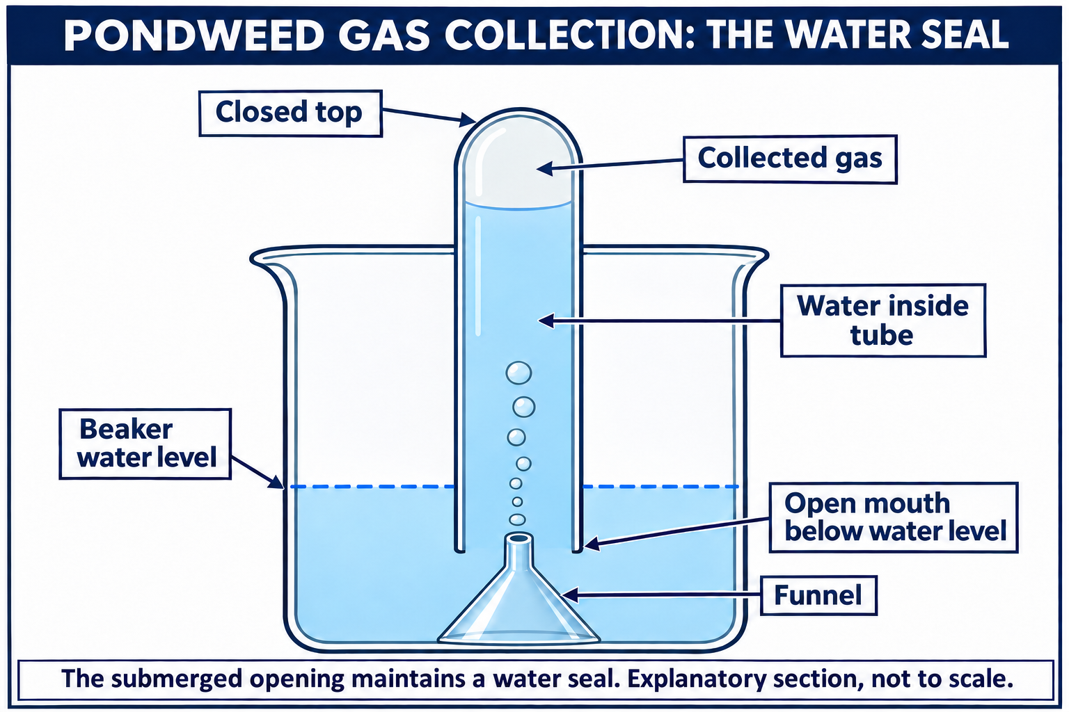
The arrangement does not establish gas purity or provide a calibrated gas-volume result.
 BIOLOGY · B16 · 3 VISUALSPhotosynthesis with dissolved oxygenUse a dissolved-oxygen sensor to follow oxygen changes around aquatic plant material.
Labelled schematic
Use a dissolved-oxygen sensor to follow oxygen changes around aquatic plant material.


Realistic apparatus view
Use a dissolved-oxygen sensor to follow oxygen changes around aquatic plant material.

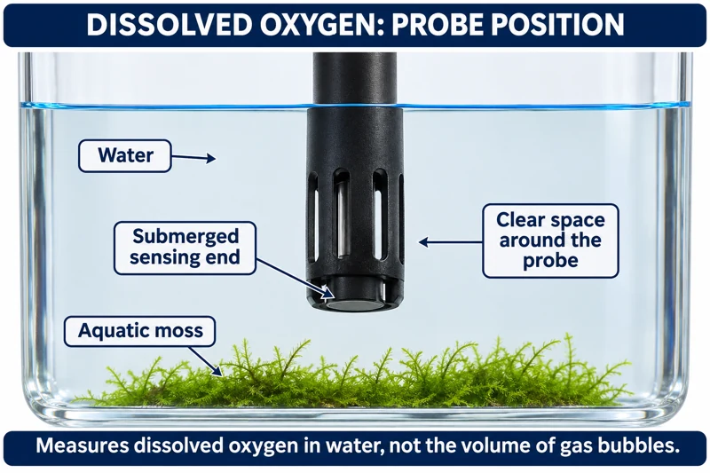
Critical detail
Use a dissolved-oxygen sensor to follow oxygen changes around aquatic plant material.

The sensor follows net oxygen balance rather than gross photosynthesis alone.
 BIOLOGY · B17 · 3 VISUALSFloating leaf discsCompare the flotation of infiltrated leaf discs under controlled light conditions.
Labelled schematic
Compare the flotation of infiltrated leaf discs under controlled light conditions.

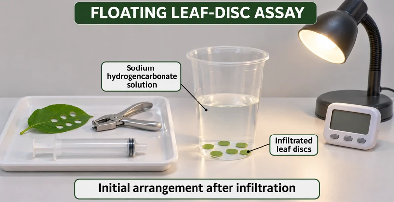
Realistic apparatus view
Compare the flotation of infiltrated leaf discs under controlled light conditions.


Critical detail
Compare the flotation of infiltrated leaf discs under controlled light conditions.
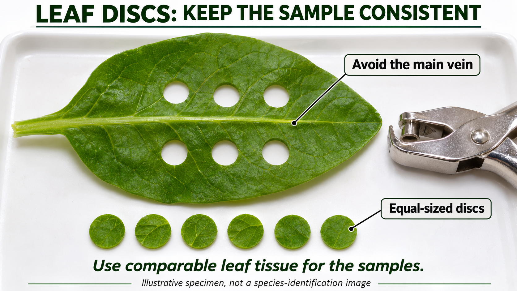
The images depict the initial sunken state after infiltration, not experimental results.
 BIOLOGY · B18 · 3 VISUALSAlgal beads and indicatorCompare indicator changes around immobilised algae in light and dark conditions.
Labelled schematic
Compare indicator changes around immobilised algae in light and dark conditions.


Realistic apparatus view
Compare indicator changes around immobilised algae in light and dark conditions.


Critical detail
Compare indicator changes around immobilised algae in light and dark conditions.

The initial colour is illustrative; changes reflect net carbon-dioxide-related activity.
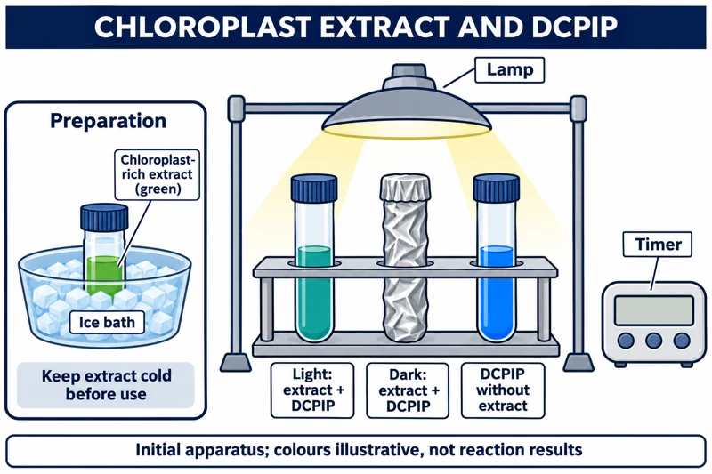 BIOLOGY · B19 · 3 VISUALSChloroplast DCPIP investigationUse DCPIP and chloroplast extract to investigate light-dependent electron-transfer activity.
Labelled schematic
Use DCPIP and chloroplast extract to investigate light-dependent electron-transfer activity.


Realistic apparatus view
Use DCPIP and chloroplast extract to investigate light-dependent electron-transfer activity.


Critical detail
Use DCPIP and chloroplast extract to investigate light-dependent electron-transfer activity.

Reduced DCPIP is colourless, but the chloroplast extract remains green; chilled preparation is separate from the reaction.
 BIOLOGY · B20 · 3 VISUALSLeaf chamber with a carbon dioxide sensorRecord carbon dioxide changes around a leaf in controlled light and dark conditions.
Labelled schematic
Record carbon dioxide changes around a leaf in controlled light and dark conditions.


Realistic apparatus view
Record carbon dioxide changes around a leaf in controlled light and dark conditions.
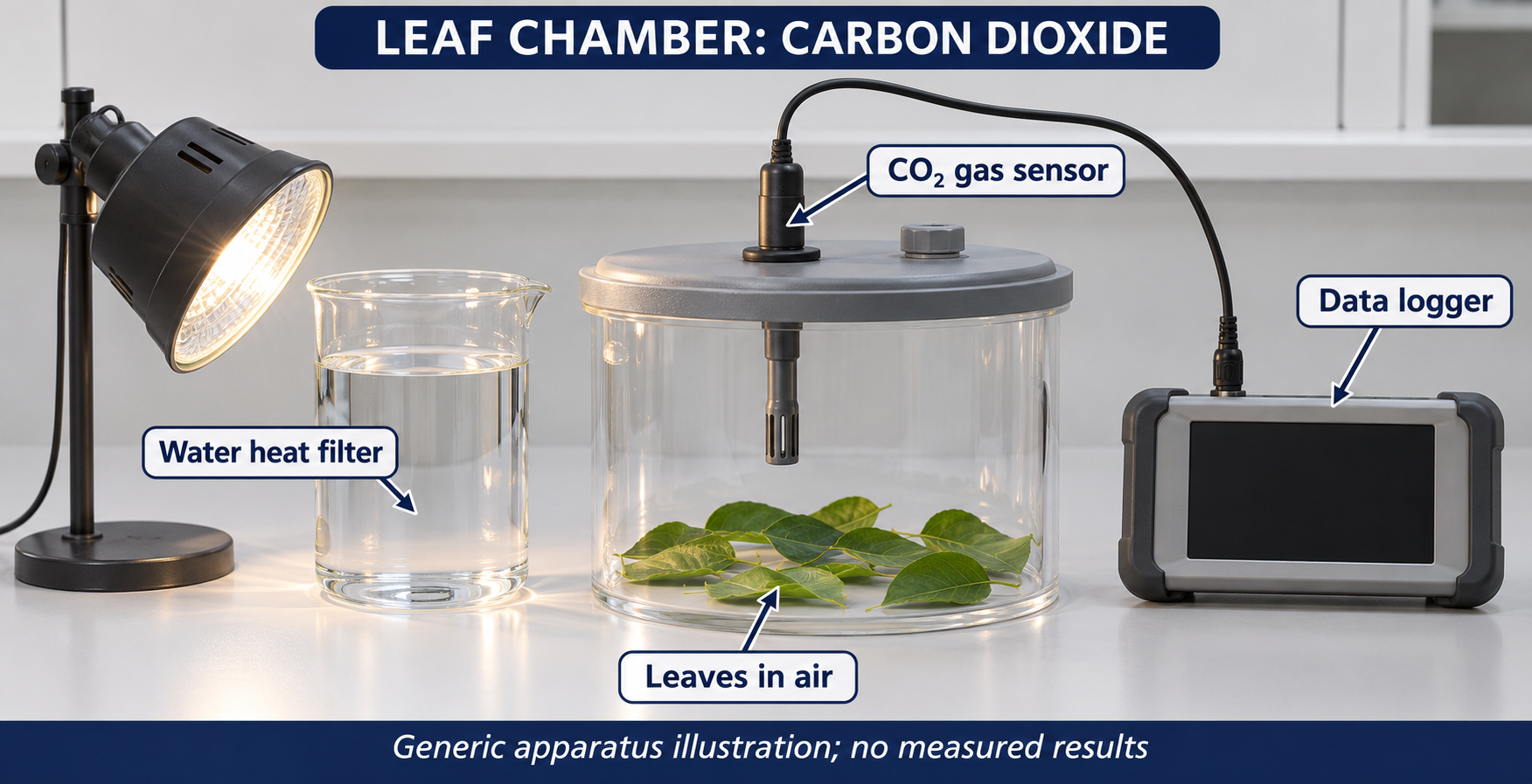

Critical detail
Record carbon dioxide changes around a leaf in controlled light and dark conditions.

The chamber measures net gas exchange, not photosynthesis independently of respiration.
 BIOLOGY · B21 · 3 VISUALSBubble potometerTrack an air bubble in a capillary to estimate water uptake by a leafy shoot.
Labelled schematic
Track an air bubble in a capillary to estimate water uptake by a leafy shoot.


Realistic apparatus view
Track an air bubble in a capillary to estimate water uptake by a leafy shoot.
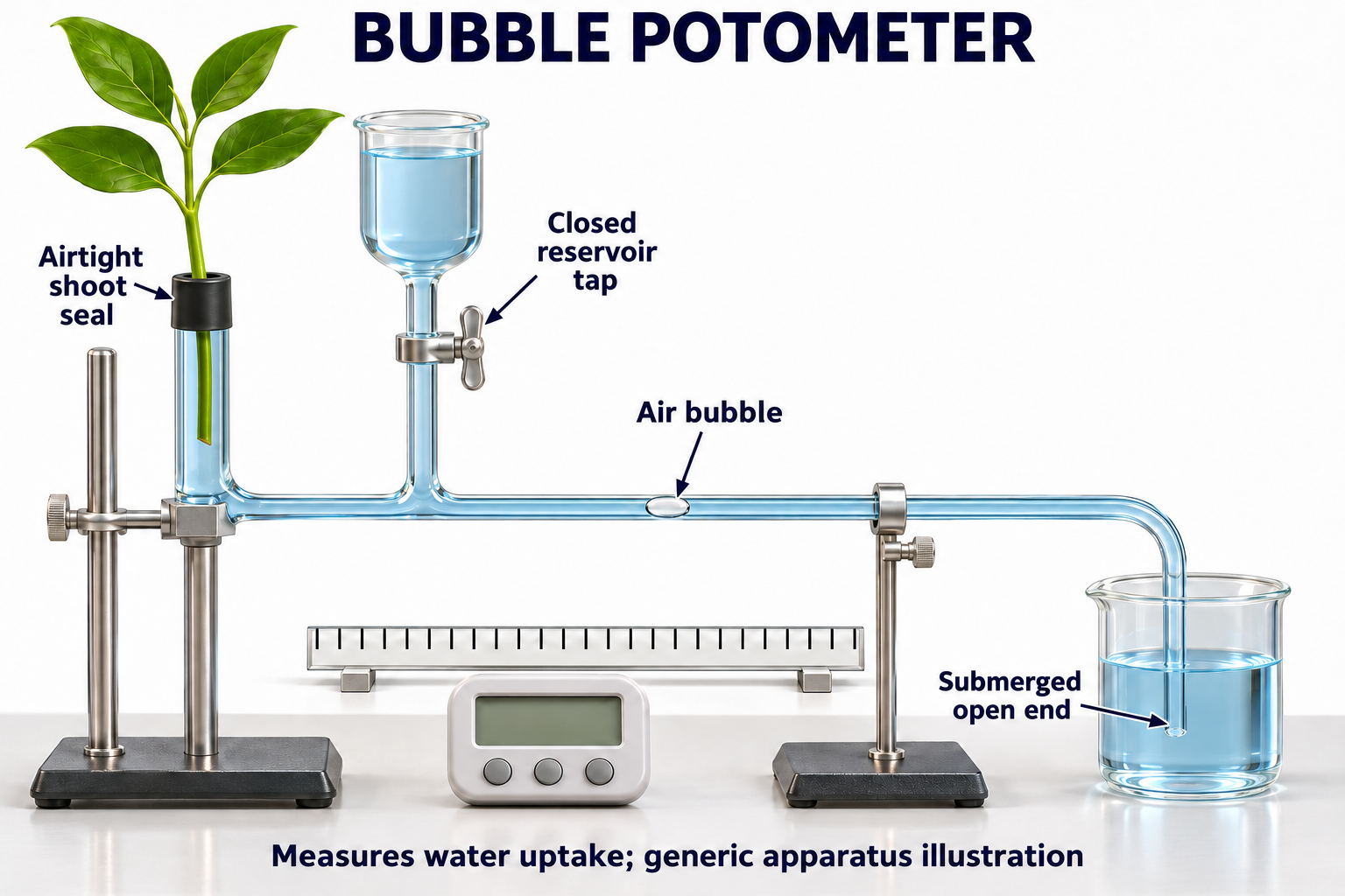
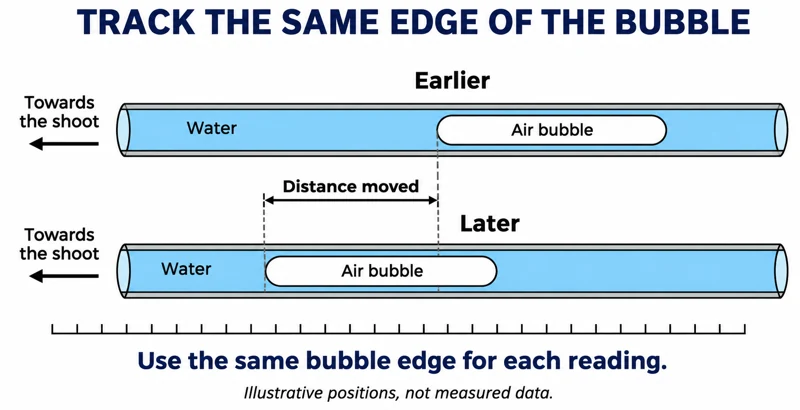
Critical detail
Track an air bubble in a capillary to estimate water uptake by a leafy shoot.

Water uptake is a proxy for transpiration; measurements should track the same bubble edge.
 BIOLOGY · B22 · 3 VISUALSPlant mass-loss transpirationUse a balance and a covered pot to follow water loss from a plant.
Labelled schematic
Use a balance and a covered pot to follow water loss from a plant.


Realistic apparatus view
Use a balance and a covered pot to follow water loss from a plant.


Critical detail
Use a balance and a covered pot to follow water loss from a plant.
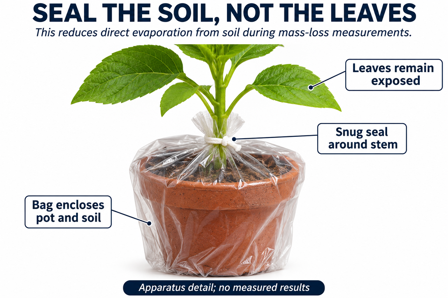
Covering the pot reduces soil evaporation but does not prove that all residual evaporation is eliminated.
 BIOLOGY · B23 · 3 VISUALSXylem dye transportTrace coloured water through a cut petiole and inspect a section.
Labelled schematic
Trace coloured water through a cut petiole and inspect a section.


Realistic apparatus view
Trace coloured water through a cut petiole and inspect a section.


Critical detail
Trace coloured water through a cut petiole and inspect a section.

The enlarged stained section is an illustration, not an authenticated micrograph.
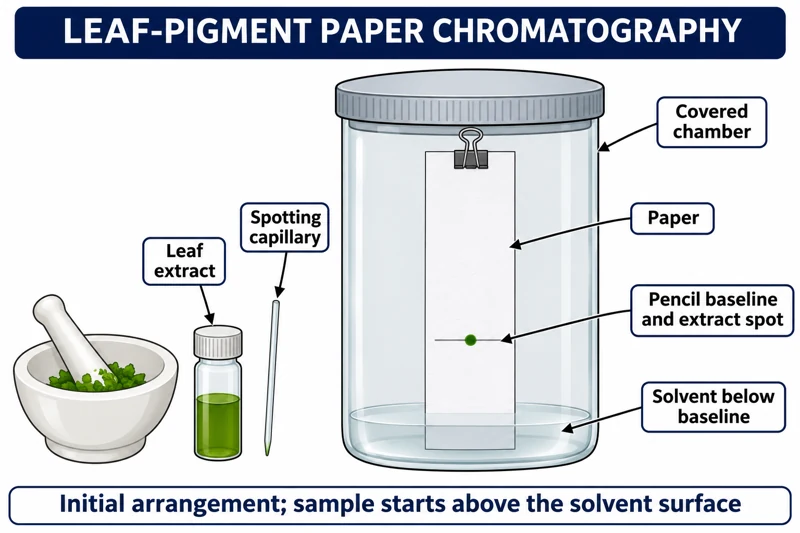 BIOLOGY · B24 · 3 VISUALSLeaf-pigment chromatographySeparate extracted leaf pigments using paper chromatography.
Labelled schematic
Separate extracted leaf pigments using paper chromatography.


Realistic apparatus view
Separate extracted leaf pigments using paper chromatography.

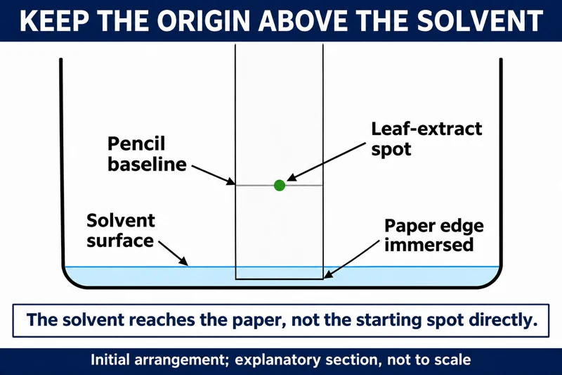
Critical detail
Separate extracted leaf pigments using paper chromatography.

The images depict initial loading above the solvent, not developed bands or measured Rf values.
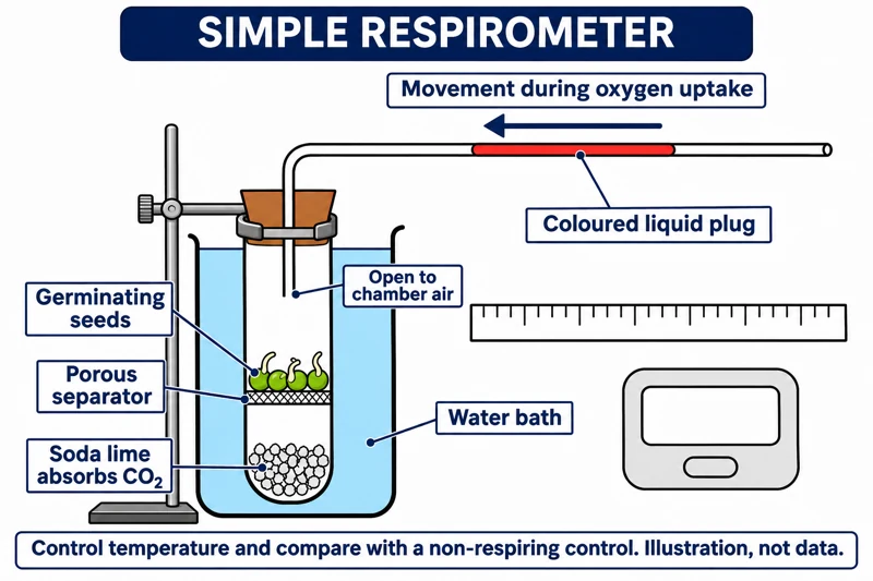 BIOLOGY · B25 · 3 VISUALSSimple respirometerEstimate oxygen uptake from movement of a liquid marker while carbon dioxide is absorbed separately.
Labelled schematic
Estimate oxygen uptake from movement of a liquid marker while carbon dioxide is absorbed separately.


Realistic apparatus view
Estimate oxygen uptake from movement of a liquid marker while carbon dioxide is absorbed separately.

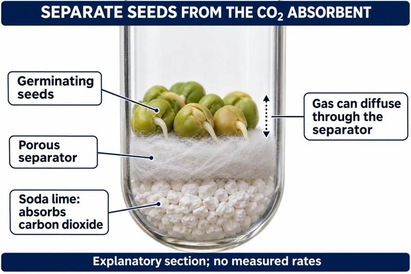
Critical detail
Estimate oxygen uptake from movement of a liquid marker while carbon dioxide is absorbed separately.

A liquid plug, suitable control and temperature stability are needed to interpret the movement.
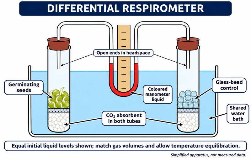 BIOLOGY · B26 · 3 VISUALSDifferential respirometerCompare respiring material with a matched control using a shared manometer and water bath.
Labelled schematic
Compare respiring material with a matched control using a shared manometer and water bath.


Realistic apparatus view
Compare respiring material with a matched control using a shared manometer and water bath.


Critical detail
Compare respiring material with a matched control using a shared manometer and water bath.

The liquid rises on the lower-pressure side; comparable chamber volumes and temperature are essential.
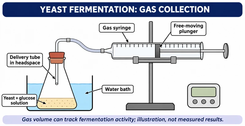 BIOLOGY · B27 · 3 VISUALSYeast fermentation and gas collectionFollow gas production from a yeast-and-glucose mixture using a gas syringe.
Labelled schematic
Follow gas production from a yeast-and-glucose mixture using a gas syringe.

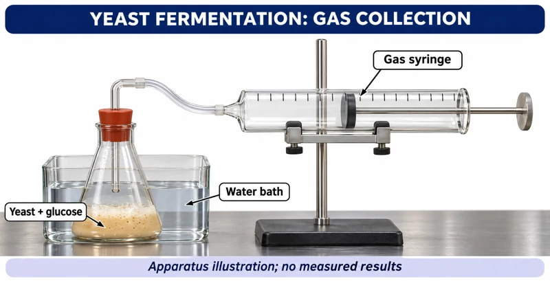
Realistic apparatus view
Follow gas production from a yeast-and-glucose mixture using a gas syringe.
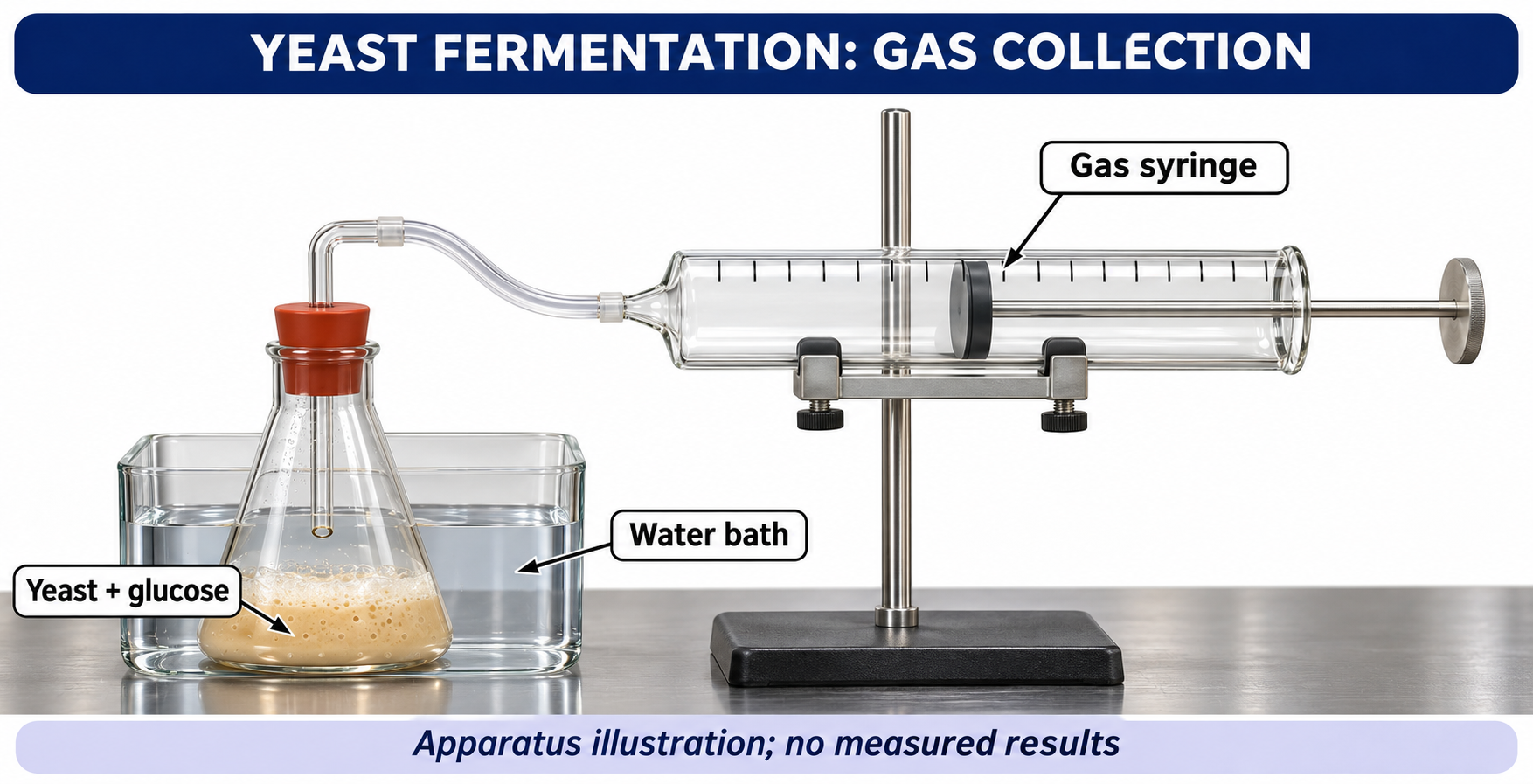
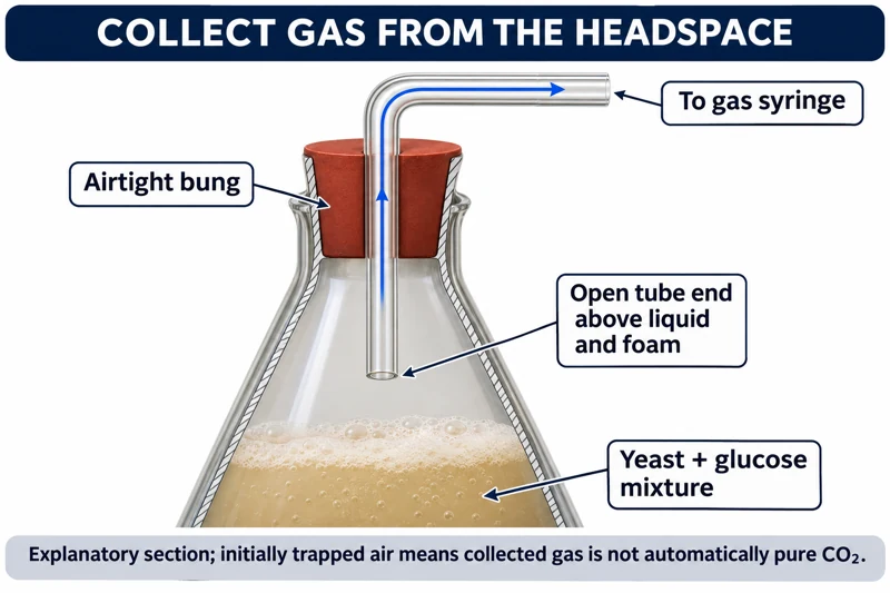
Critical detail
Follow gas production from a yeast-and-glucose mixture using a gas syringe.

Trapped air means the collected gas is not necessarily pure carbon dioxide or evidence of oxygen-free conditions.
 BIOLOGY · B28 · 3 VISUALSRespiration gas-sensor chamberRecord gas concentration changes around respiring seeds with a sensor.
Labelled schematic
Record gas concentration changes around respiring seeds with a sensor.
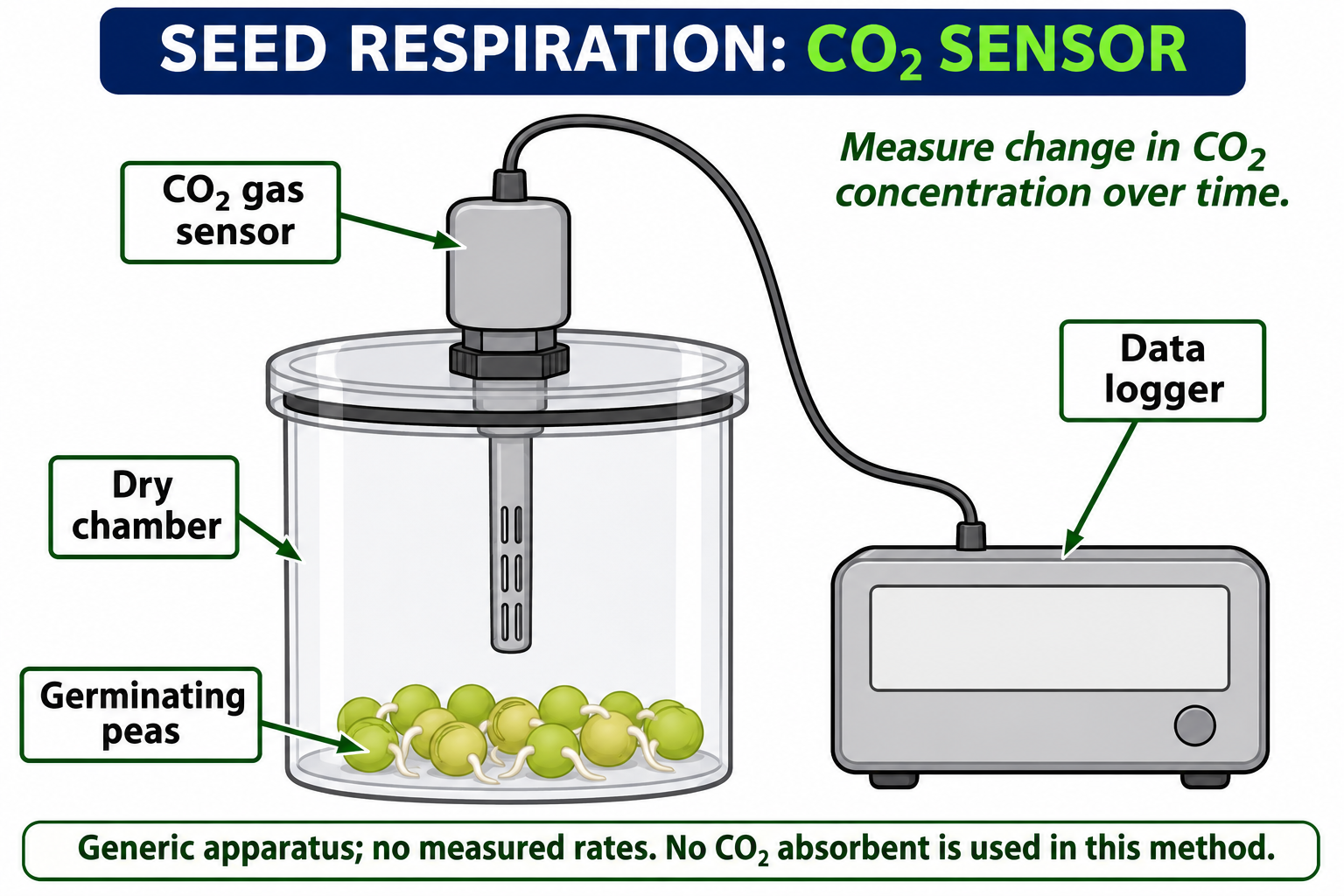
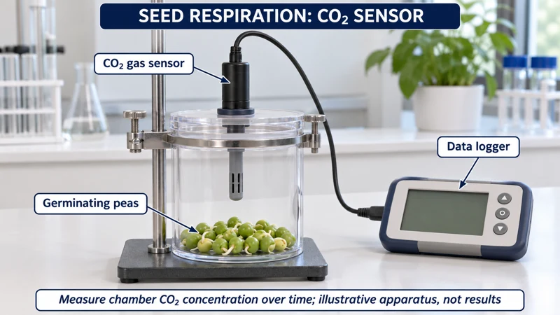
Realistic apparatus view
Record gas concentration changes around respiring seeds with a sensor.
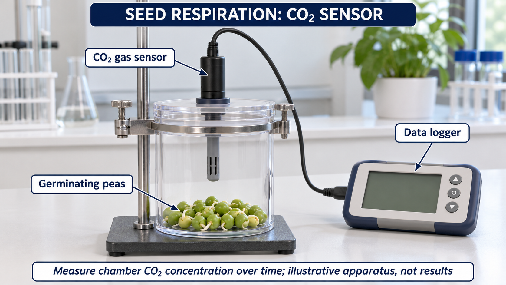
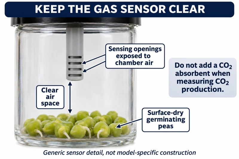
Critical detail
Record gas concentration changes around respiring seeds with a sensor.

Concentration change is not a calibrated respiration rate without chamber-volume and time information.
 BIOLOGY · B29 · 3 VISUALSHeat release from germinating seedsCompare temperatures in insulated seed vessels to investigate heat release during respiration.
Labelled schematic
Compare temperatures in insulated seed vessels to investigate heat release during respiration.


Realistic apparatus view
Compare temperatures in insulated seed vessels to investigate heat release during respiration.


Critical detail
Compare temperatures in insulated seed vessels to investigate heat release during respiration.

Start with matched temperatures and interpret the treatment against its control.
 BIOLOGY · B30 · 3 VISUALSSpirometry with a flow sensorRecord breathing airflow using a generic flow-head sensor and data logger.
Labelled schematic
Record breathing airflow using a generic flow-head sensor and data logger.


Realistic apparatus view
Record breathing airflow using a generic flow-head sensor and data logger.
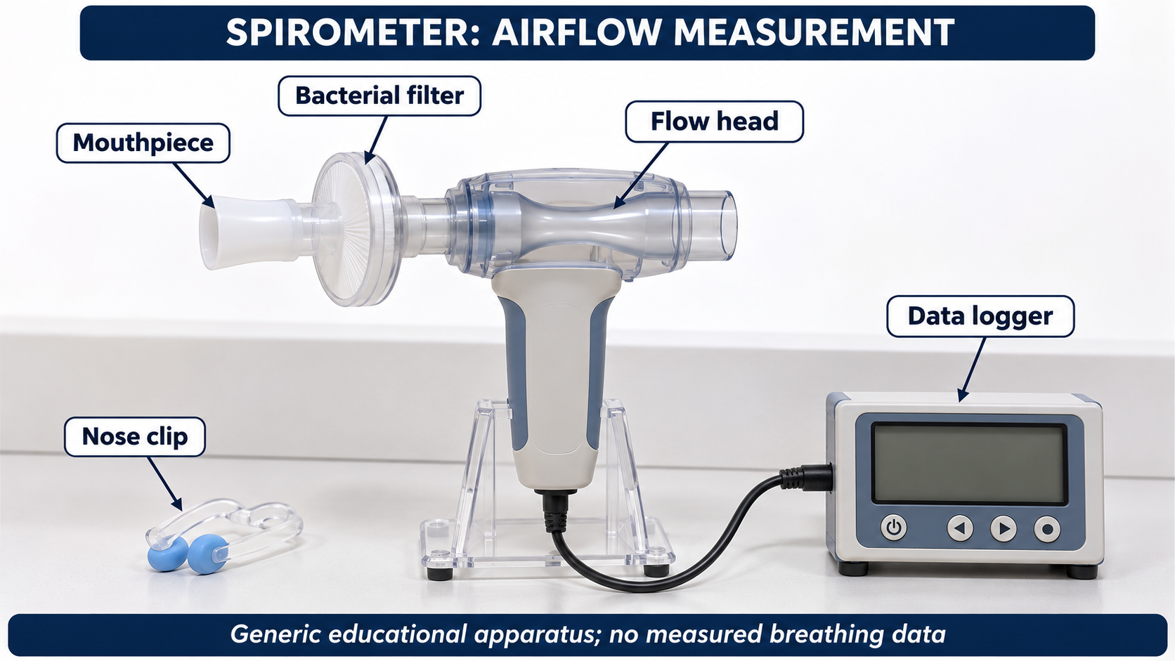

Critical detail
Record breathing airflow using a generic flow-head sensor and data logger.

The apparatus is conceptual rather than a specific manufacturer's assembly; no clinical trace is provided.
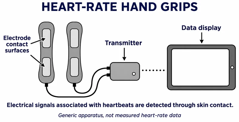 BIOLOGY · B31 · 3 VISUALSHeart-rate hand-grip sensorRecord heart-rate signals using electrical hand grips and a data logger.
Labelled schematic
Record heart-rate signals using electrical hand grips and a data logger.


Realistic apparatus view
Record heart-rate signals using electrical hand grips and a data logger.

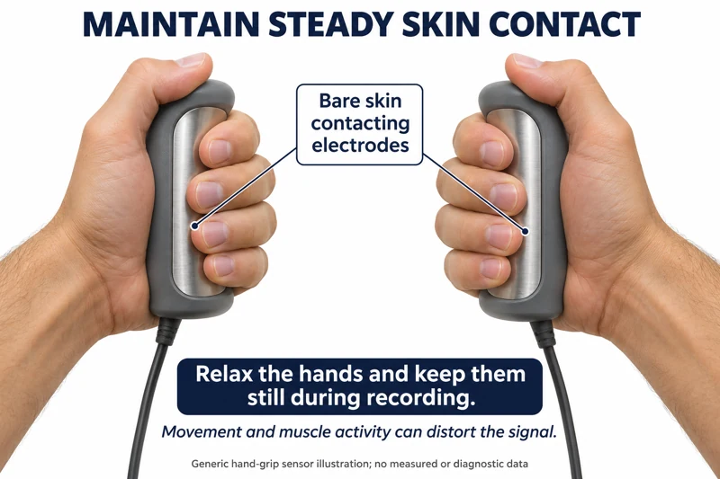
Critical detail
Record heart-rate signals using electrical hand grips and a data logger.

Movement and muscle activity can introduce artefacts; the illustration is not a diagnostic measurement.
 BIOLOGY · B32 · 3 VISUALSRandom quadrat samplingUse randomly selected coordinates to position quadrats when estimating plant abundance or cover.
Labelled schematic
Use randomly selected coordinates to position quadrats when estimating plant abundance or cover.


Realistic apparatus view
Use randomly selected coordinates to position quadrats when estimating plant abundance or cover.
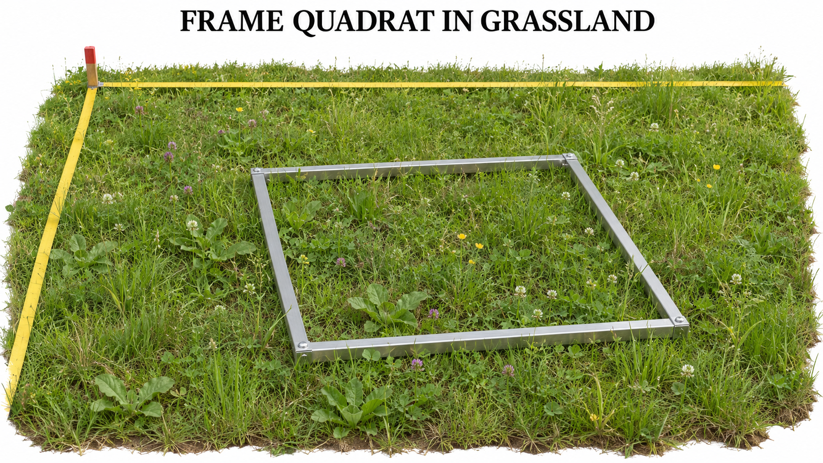

Critical detail
Use randomly selected coordinates to position quadrats when estimating plant abundance or cover.
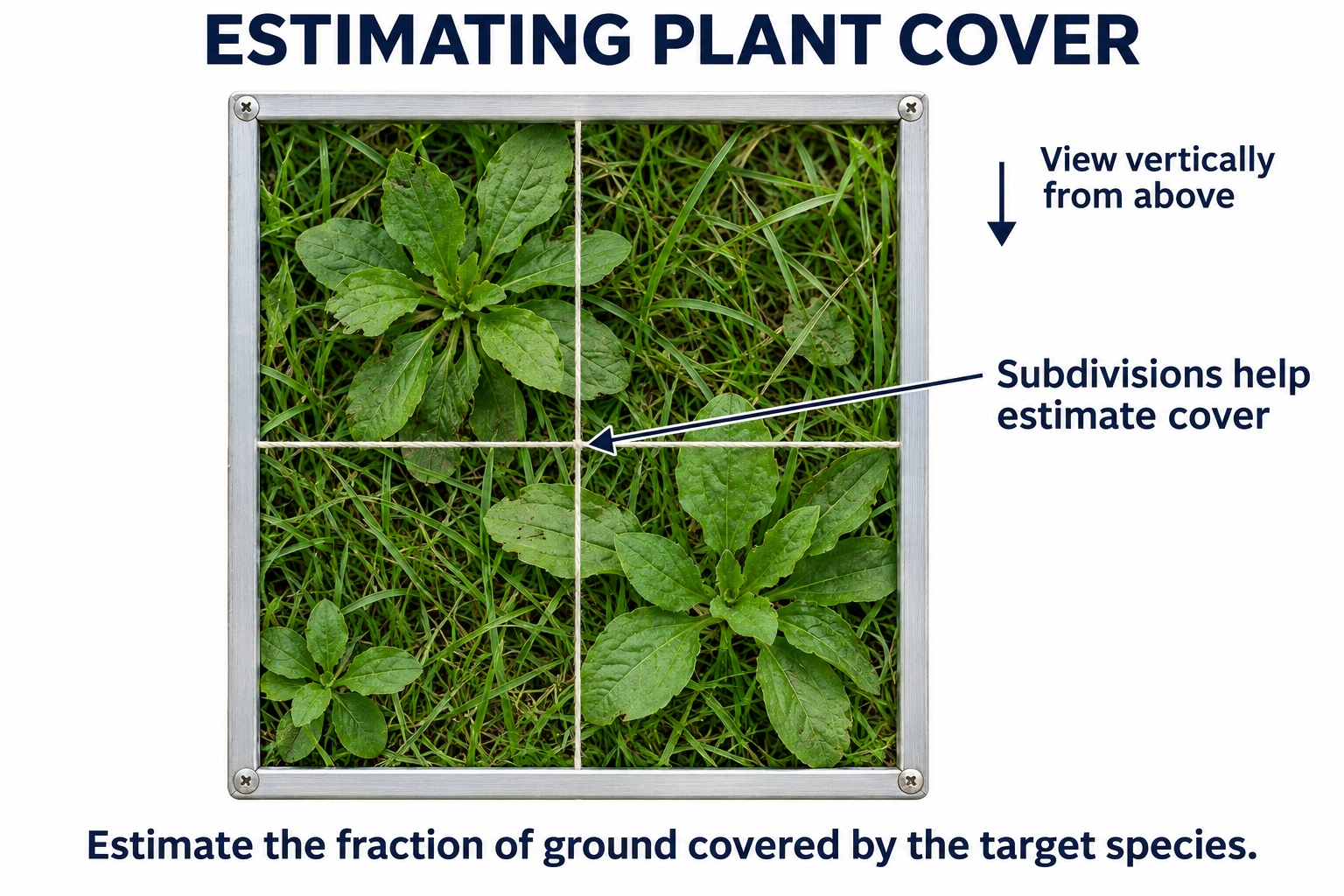
Plants and sample placements are illustrative, not a validated species survey or sufficient sample size.
 BIOLOGY · B33 · 3 VISUALSInterrupted belt transectPlace quadrats at intervals along a transect to investigate species distribution.
Labelled schematic
Place quadrats at intervals along a transect to investigate species distribution.


Realistic apparatus view
Place quadrats at intervals along a transect to investigate species distribution.
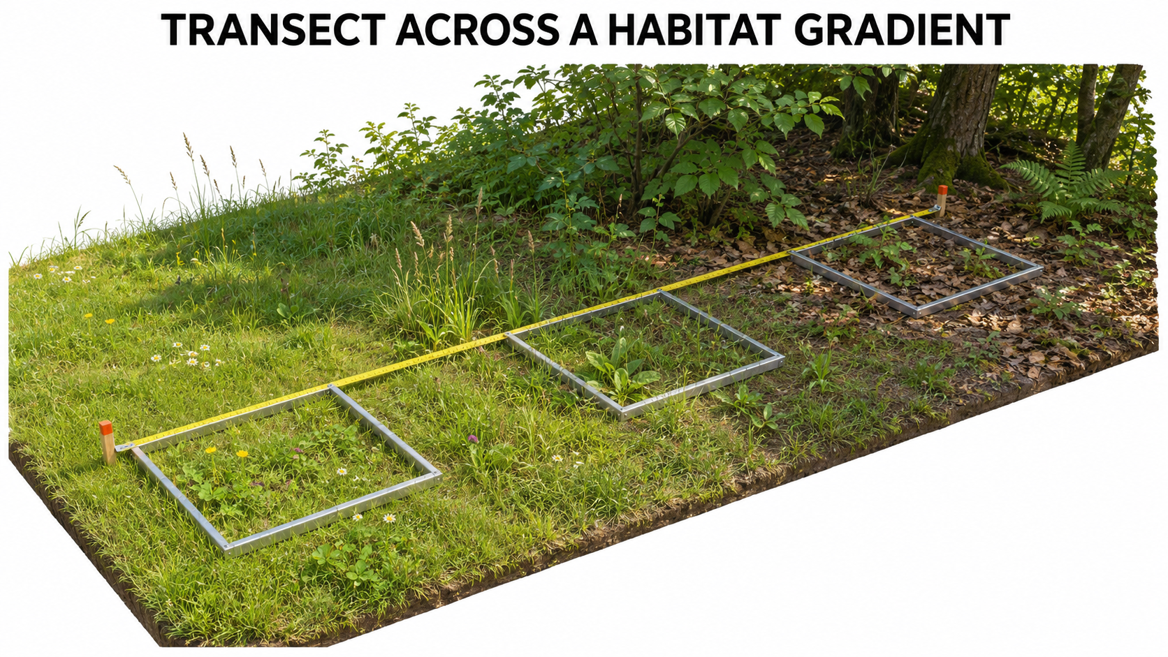

Critical detail
Place quadrats at intervals along a transect to investigate species distribution.

The diagram illustrates consistent placement, not sufficient replication for an ecological conclusion.
 BIOLOGY · B34 · 3 VISUALSChoice chamberCompare invertebrate positions in a chamber offering controlled environmental contrasts.
Labelled schematic
Compare invertebrate positions in a chamber offering controlled environmental contrasts.


Realistic apparatus view
Compare invertebrate positions in a chamber offering controlled environmental contrasts.


Critical detail
Compare invertebrate positions in a chamber offering controlled environmental contrasts.

The starting arrangement contains no preference result; other conditions such as humidity and temperature must be matched.
 BIOLOGY · B35 · 3 VISUALSPhototropism chamberExpose seedlings to directional light through a single opening to investigate growth responses.
Labelled schematic
Expose seedlings to directional light through a single opening to investigate growth responses.
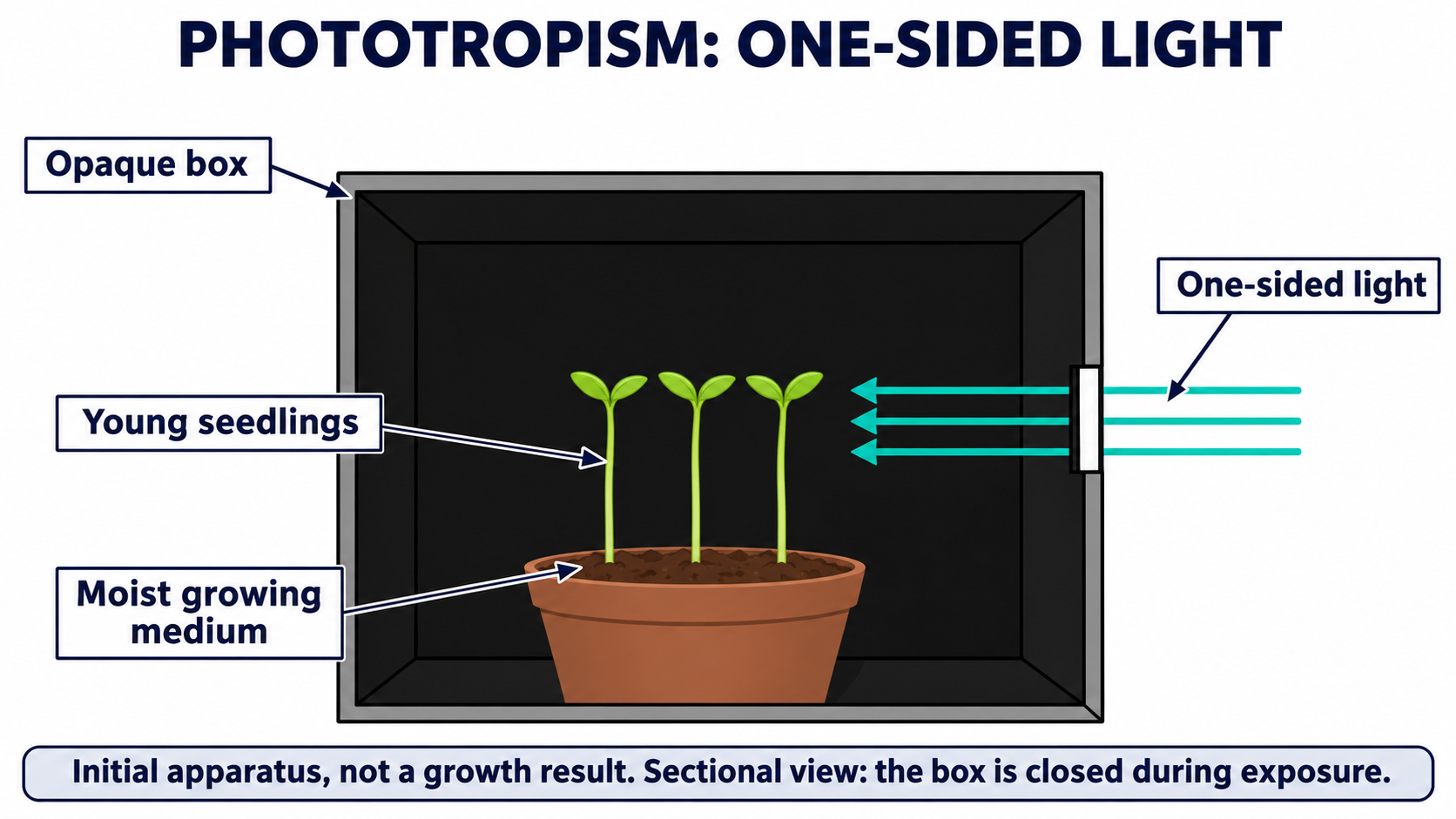

Realistic apparatus view
Expose seedlings to directional light through a single opening to investigate growth responses.

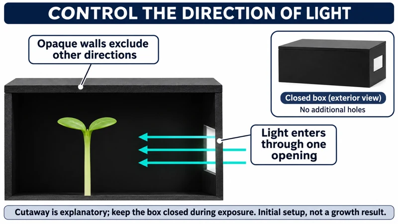
Critical detail
Expose seedlings to directional light through a single opening to investigate growth responses.
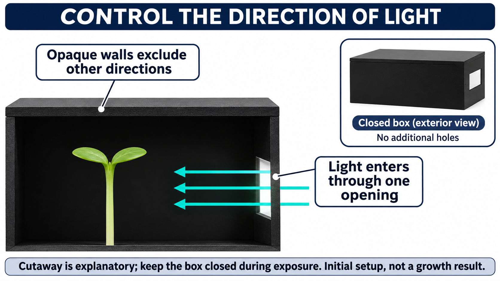
The front cutaway reveals an otherwise opaque enclosure; no growth outcome is shown.
 BIOLOGY · B36 · 3 VISUALSSeed germination comparisonCompare seeds on moist and dry paper to investigate the role of water in germination.
Labelled schematic
Compare seeds on moist and dry paper to investigate the role of water in germination.
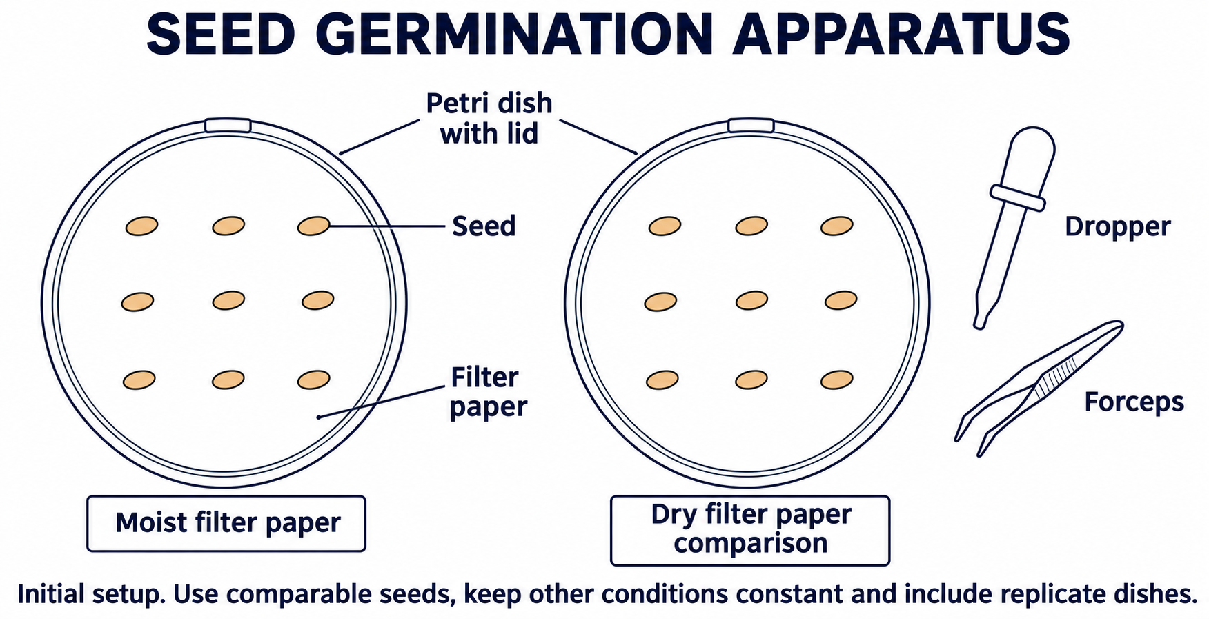
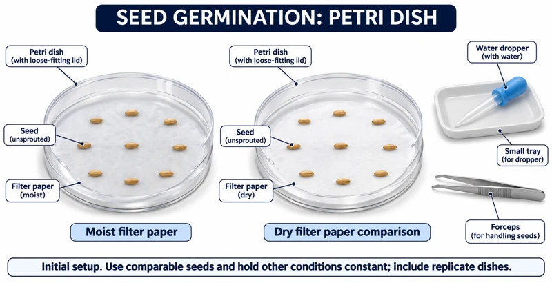
Realistic apparatus view
Compare seeds on moist and dry paper to investigate the role of water in germination.


Critical detail
Compare seeds on moist and dry paper to investigate the role of water in germination.

The seeds are shown before germination; the layout does not establish sufficient replication.
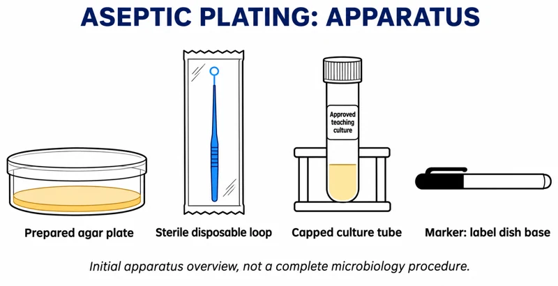 BIOLOGY · B37 · 3 VISUALSAseptic plating workstationShow the initial equipment arrangement for handling approved teaching cultures and agar plates.
Labelled schematic
Show the initial equipment arrangement for handling approved teaching cultures and agar plates.


Realistic apparatus view
Show the initial equipment arrangement for handling approved teaching cultures and agar plates.


Critical detail
Show the initial equipment arrangement for handling approved teaching cultures and agar plates.
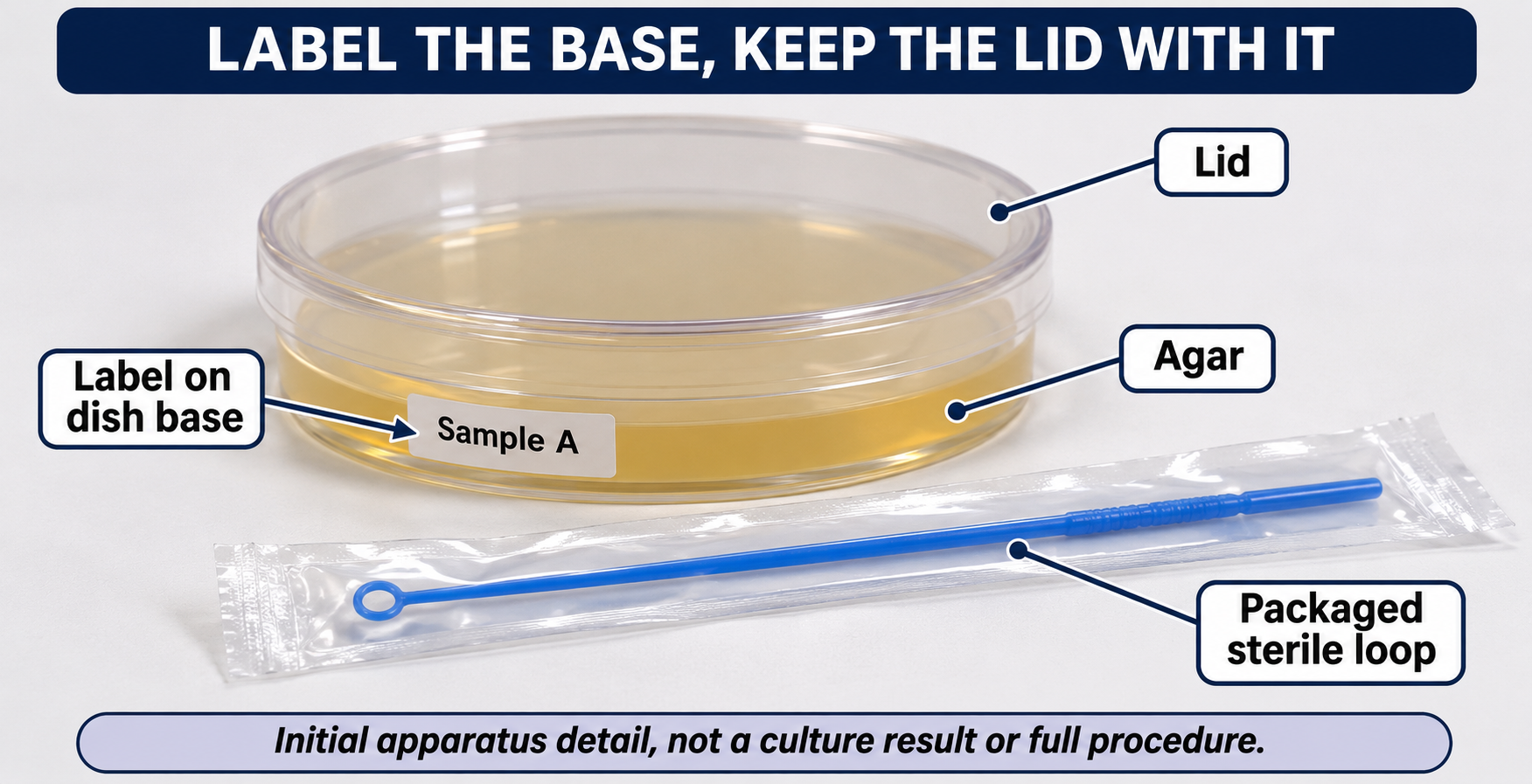
The closed plate and packaged loop depict preparation only, not incubation, results or a complete method.
 BIOLOGY · B38 · 3 VISUALSOnion DNA extractionShow the equipment used to prepare and layer an onion extract for crude DNA extraction.
Labelled schematic
Show the equipment used to prepare and layer an onion extract for crude DNA extraction.


Realistic apparatus view
Show the equipment used to prepare and layer an onion extract for crude DNA extraction.


Critical detail
Show the equipment used to prepare and layer an onion extract for crude DNA extraction.
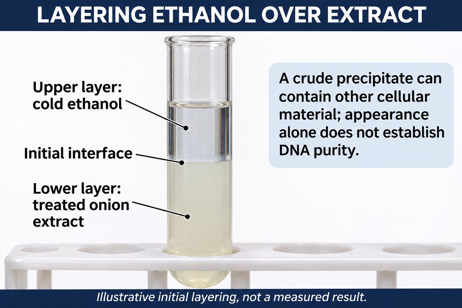
The material is not purified DNA, and the illustration does not authenticate a visible precipitate.
 BIOLOGY · B39 · 3 VISUALSDNA gel electrophoresisLoad DNA samples into an agarose gel and separate fragments using an electric field.
Labelled schematic
Load DNA samples into an agarose gel and separate fragments using an electric field.


Realistic apparatus view
Load DNA samples into an agarose gel and separate fragments using an electric field.


Critical detail
Load DNA samples into an agarose gel and separate fragments using an electric field.
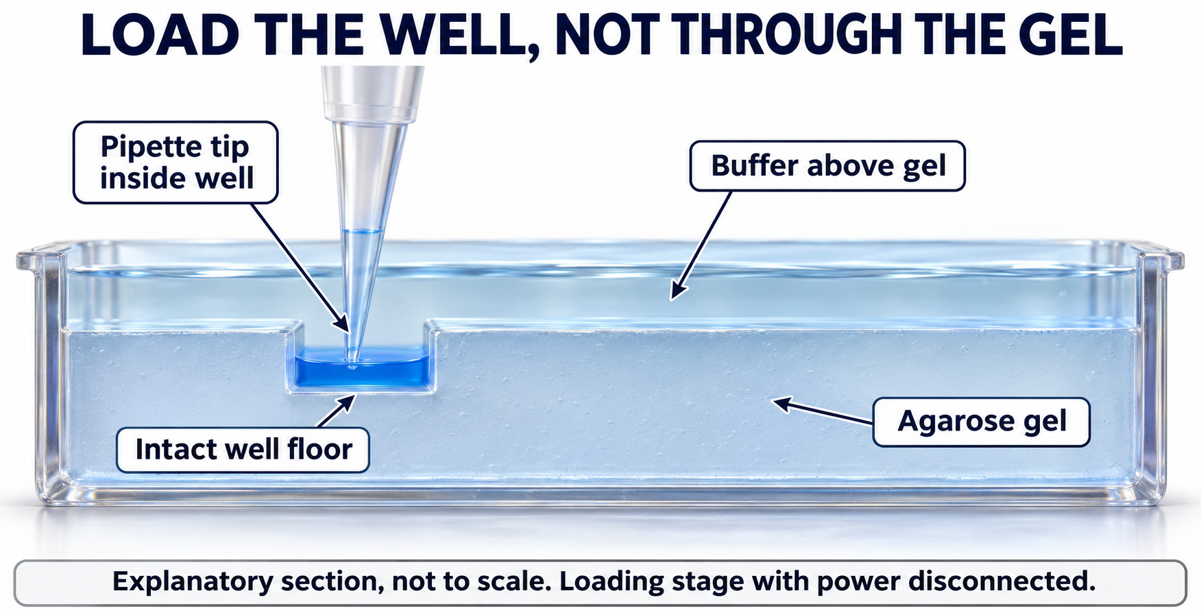
Wells are placed at the negative end so DNA migrates toward the positive electrode; the images are not experimental band data.
 BIOLOGY · B40 · 3 VISUALSPCR workstationArrange tubes and a thermal cycler for amplification of a selected DNA region.
Labelled schematic
Arrange tubes and a thermal cycler for amplification of a selected DNA region.


Realistic apparatus view
Arrange tubes and a thermal cycler for amplification of a selected DNA region.
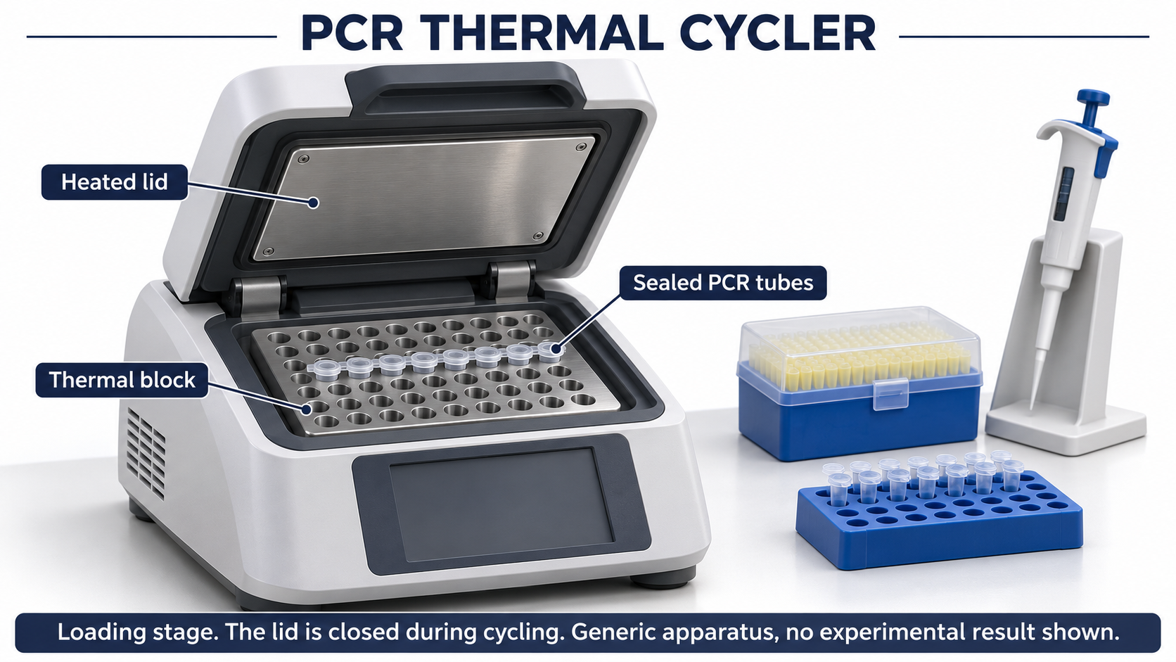
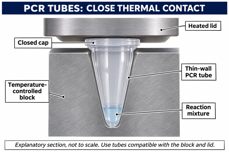
Critical detail
Arrange tubes and a thermal cycler for amplification of a selected DNA region.
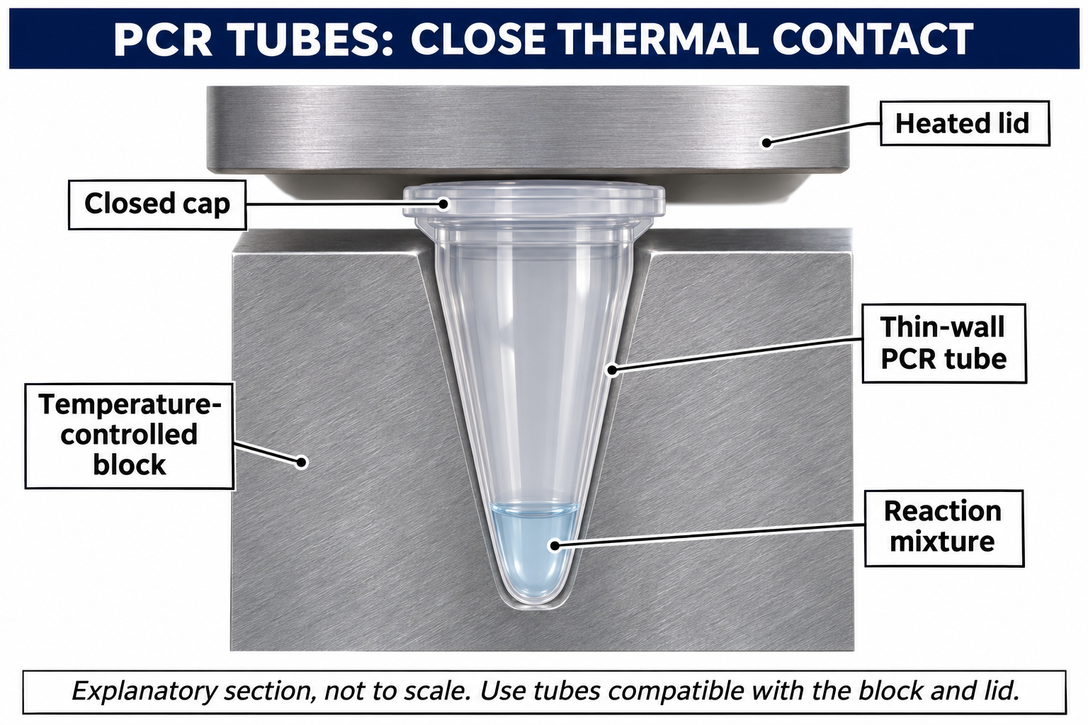
The generic heated-lid and block view shows initial loading, not active cycling or amplification data.
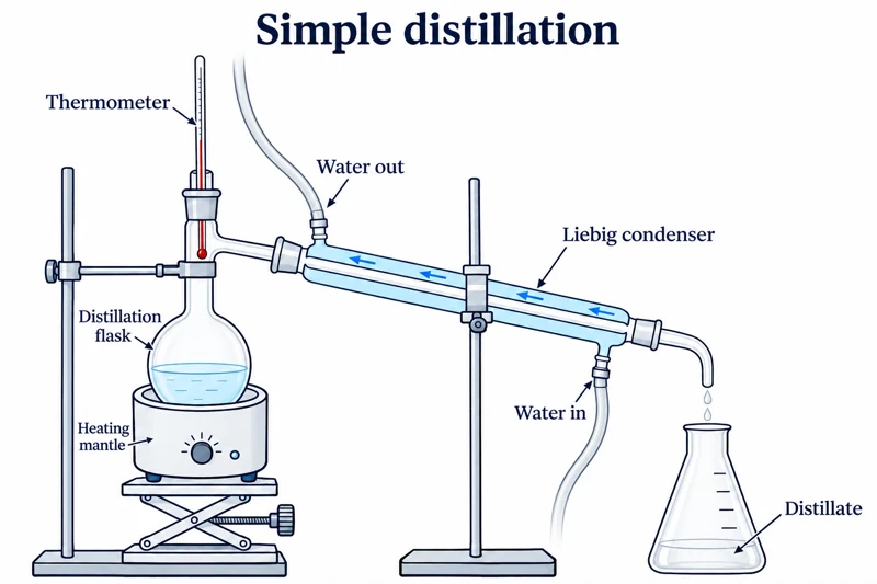 CHEMISTRY · C01 · 3 VISUALSSimple distillationSeparate a volatile liquid from less volatile material using a heated flask, condenser and receiver.
Labelled schematic
Separate a volatile liquid from less volatile material using a heated flask, condenser and receiver.

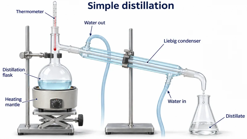
Realistic apparatus view
Separate a volatile liquid from less volatile material using a heated flask, condenser and receiver.
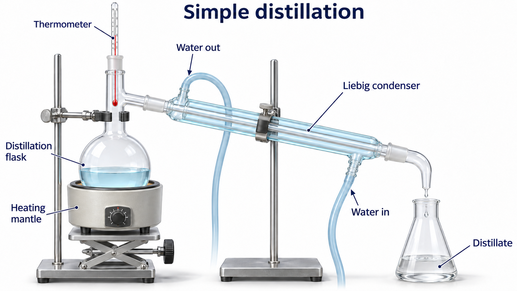
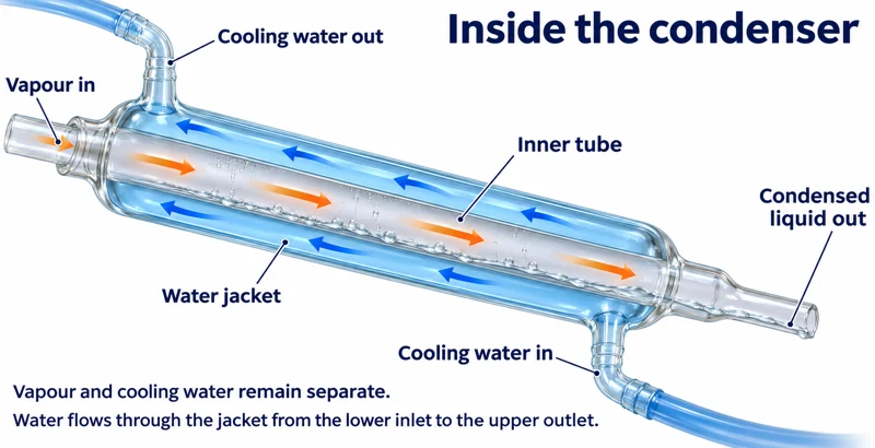
Critical detail
Separate a volatile liquid from less volatile material using a heated flask, condenser and receiver.
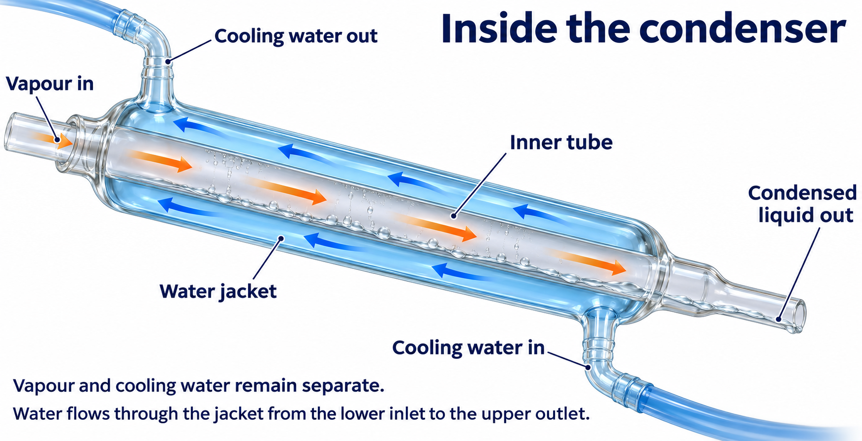
The apparatus is illustrative rather than a calibrated temperature or scale reference.
 CHEMISTRY · C02 · 3 VISUALSFractional distillationUse a fractionating column to improve separation of miscible liquids with different volatilities.
Labelled schematic
Use a fractionating column to improve separation of miscible liquids with different volatilities.


Realistic apparatus view
Use a fractionating column to improve separation of miscible liquids with different volatilities.


Critical detail
Use a fractionating column to improve separation of miscible liquids with different volatilities.
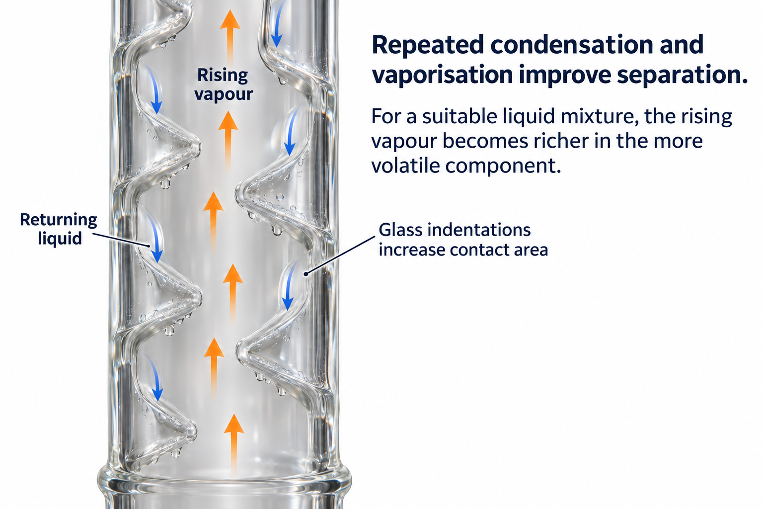
The Vigreux-column detail is stylised and does not imply a particular separation efficiency.
 CHEMISTRY · C03 · 3 VISUALSHeating under refluxHeat a reaction while condensed vapour returns to the same flask.
Labelled schematic
Heat a reaction while condensed vapour returns to the same flask.


Realistic apparatus view
Heat a reaction while condensed vapour returns to the same flask.
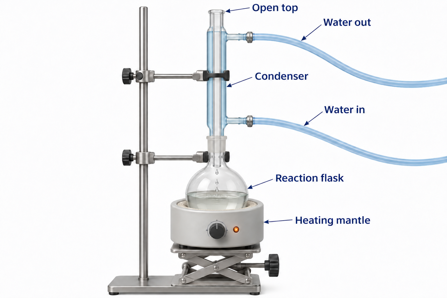

Critical detail
Heat a reaction while condensed vapour returns to the same flask.

The condenser has an open vapour path; this is not a sealed pressure system.
 CHEMISTRY · C04 · 3 VISUALSReflux with controlled additionIntroduce a reagent through an addition funnel while a reaction is heated under reflux.
Labelled schematic
Introduce a reagent through an addition funnel while a reaction is heated under reflux.


Realistic apparatus view
Introduce a reagent through an addition funnel while a reaction is heated under reflux.
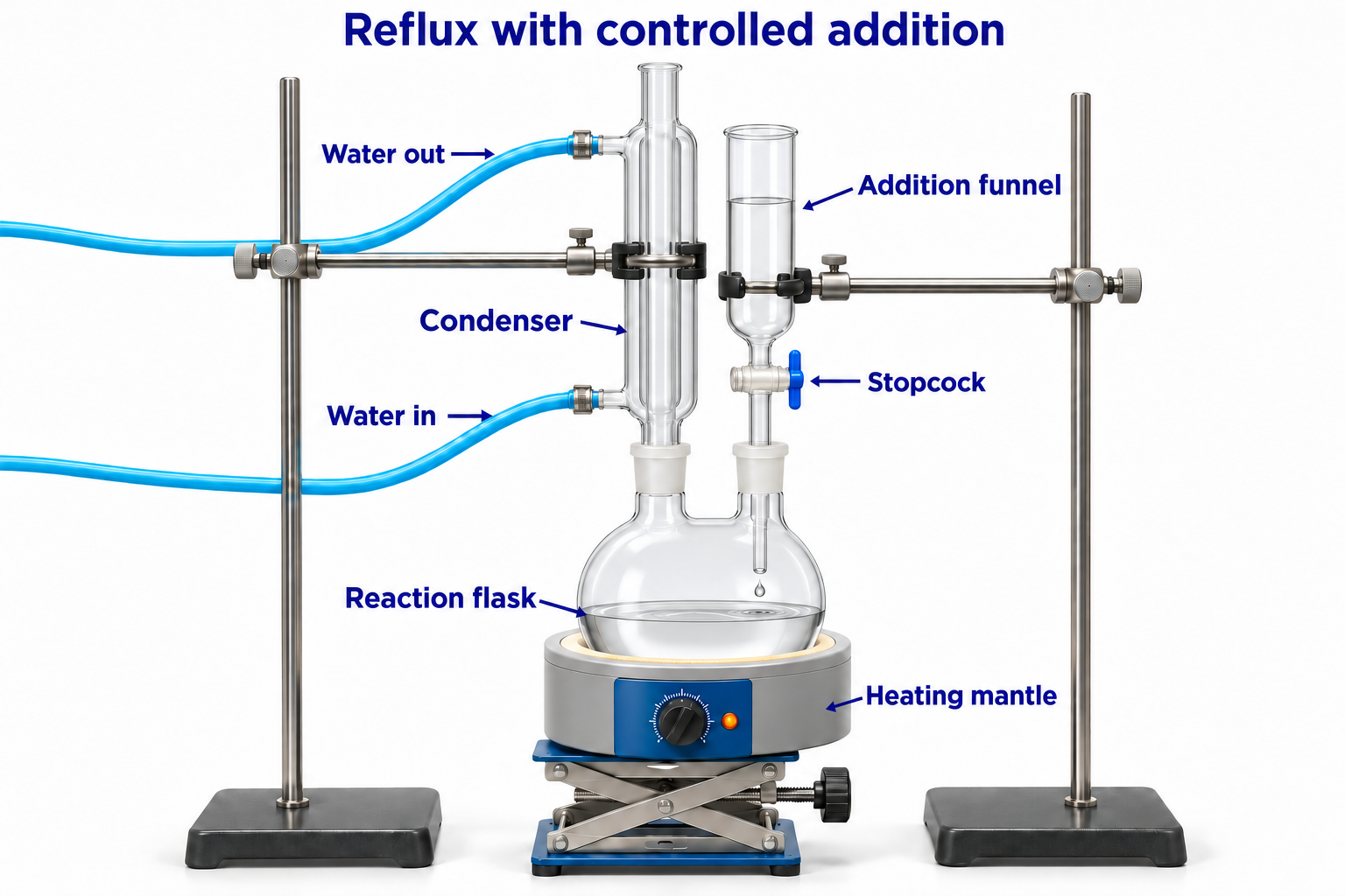

Critical detail
Introduce a reagent through an addition funnel while a reaction is heated under reflux.
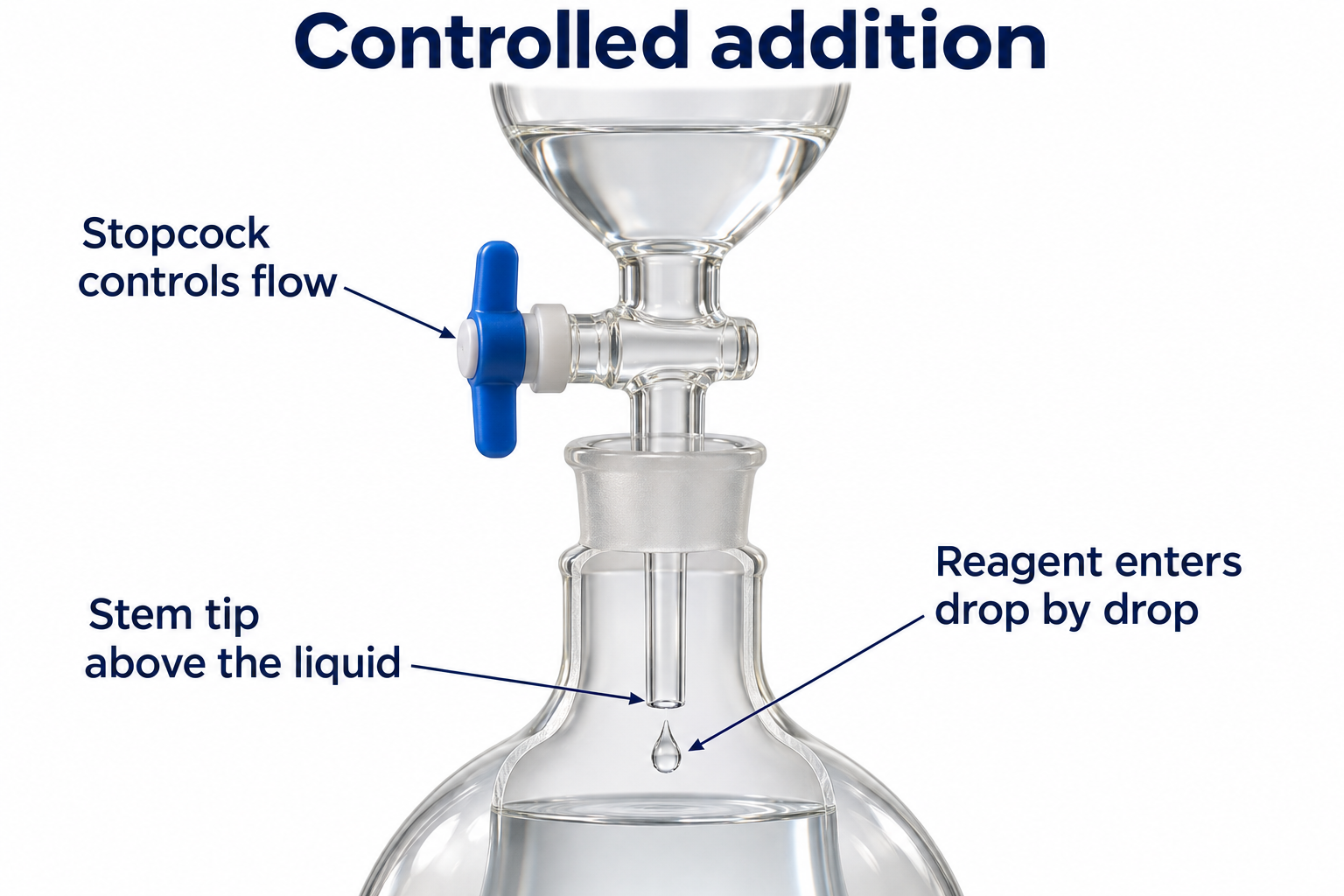
The images illustrate the glassware arrangement rather than a specified reaction or addition rate.
 CHEMISTRY · C05 · 3 VISUALSHydrodistillationDistil suitable volatile plant components with water and collect the condensate.
Labelled schematic
Distil suitable volatile plant components with water and collect the condensate.


Realistic apparatus view
Distil suitable volatile plant components with water and collect the condensate.
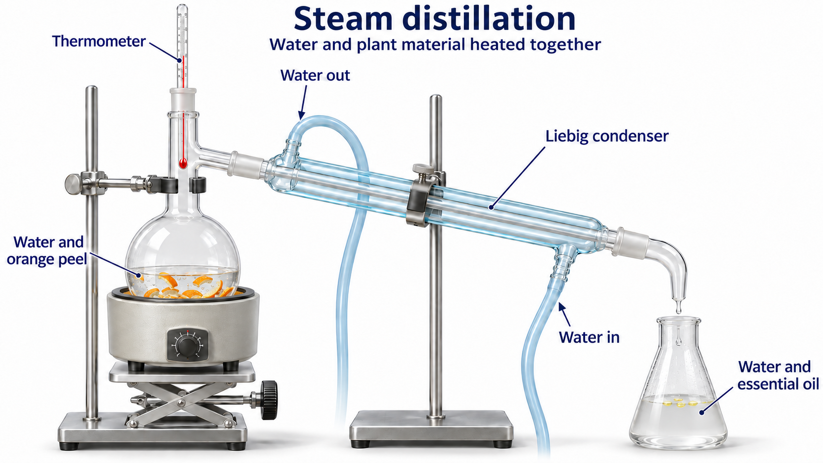

Critical detail
Distil suitable volatile plant components with water and collect the condensate.
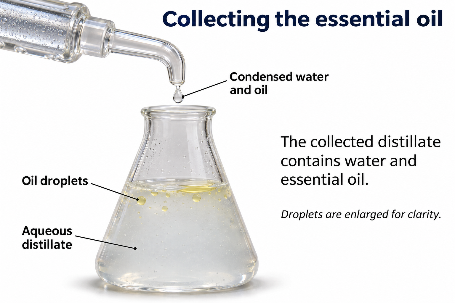
This is the hydrodistillation variant, with water in the heated flask, not a separate steam-generator setup.
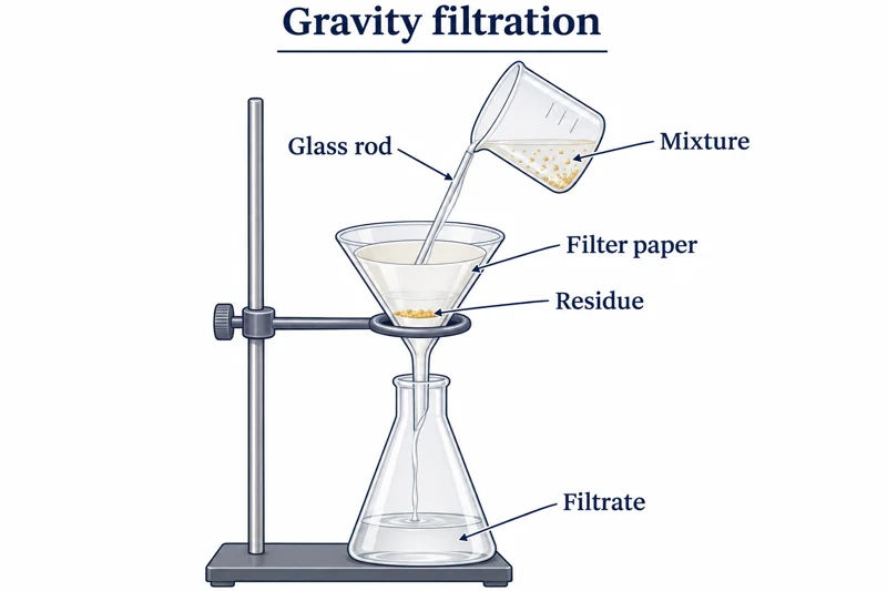 CHEMISTRY · C06 · 3 VISUALSGravity filtrationSeparate an insoluble solid from a liquid using filter paper and a funnel.
Labelled schematic
Separate an insoluble solid from a liquid using filter paper and a funnel.


Realistic apparatus view
Separate an insoluble solid from a liquid using filter paper and a funnel.


Critical detail
Separate an insoluble solid from a liquid using filter paper and a funnel.
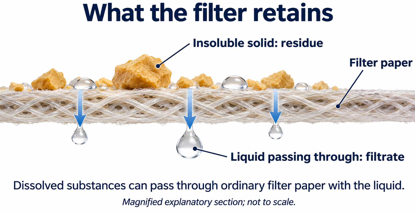
The enlarged paper section is conceptual and is not a scale drawing of pore size.
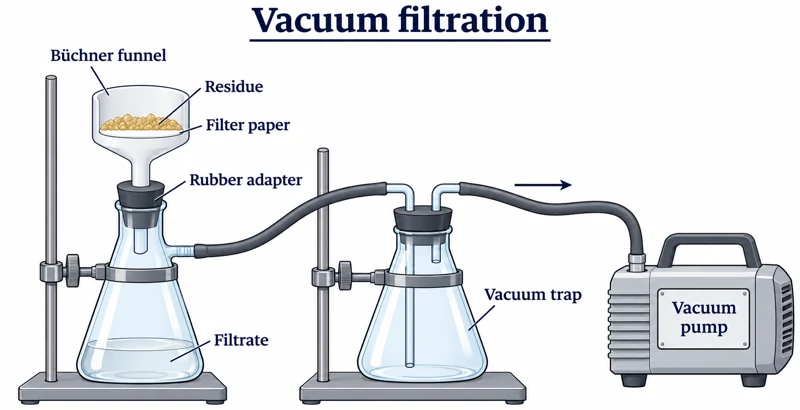 CHEMISTRY · C07 · 3 VISUALSVacuum filtrationCollect a solid using a supported filter funnel and reduced pressure.
Labelled schematic
Collect a solid using a supported filter funnel and reduced pressure.


Realistic apparatus view
Collect a solid using a supported filter funnel and reduced pressure.


Critical detail
Collect a solid using a supported filter funnel and reduced pressure.

The images show apparatus connections rather than a specified filtration pressure or flow rate.
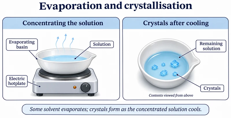 CHEMISTRY · C08 · 3 VISUALSEvaporation and crystallisationConcentrate a suitable salt solution and allow crystals to form.
Labelled schematic
Concentrate a suitable salt solution and allow crystals to form.
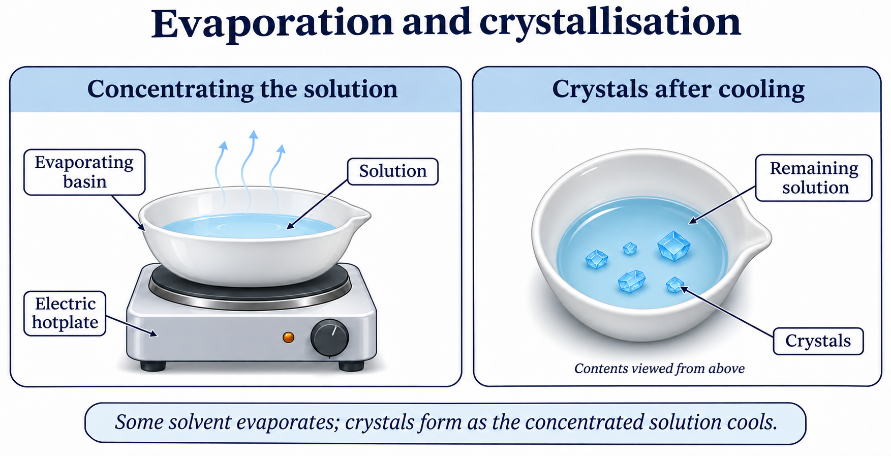

Realistic apparatus view
Concentrate a suitable salt solution and allow crystals to form.


Critical detail
Concentrate a suitable salt solution and allow crystals to form.
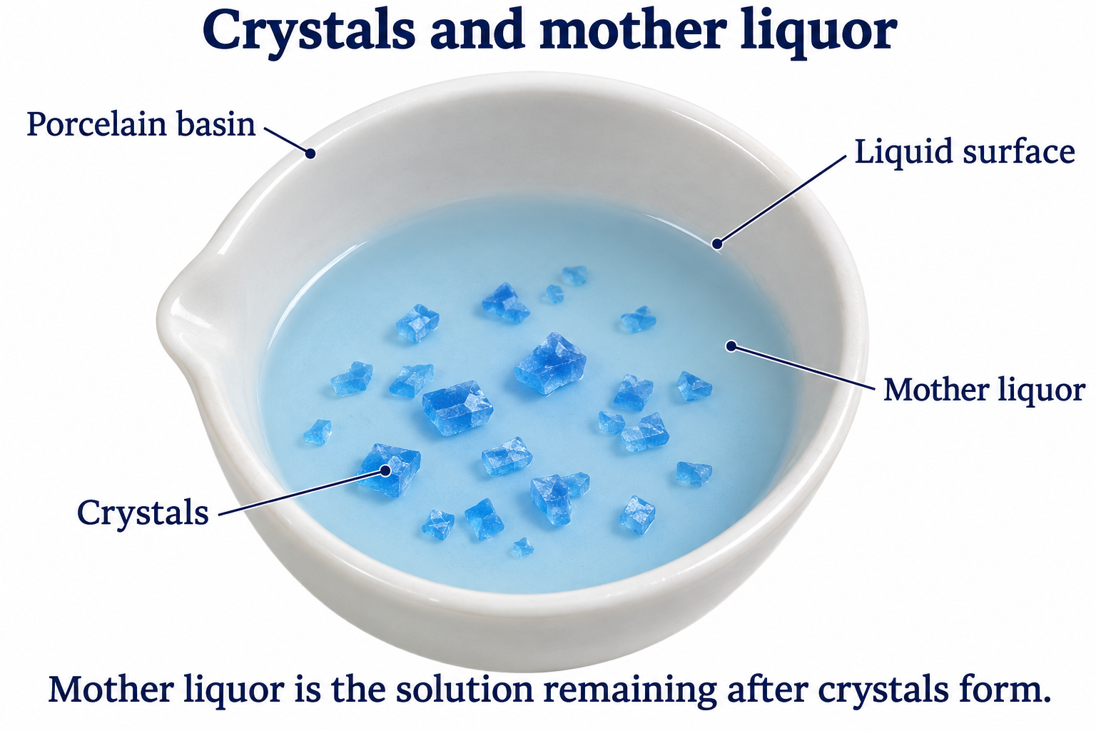
Crystal colour and habit are illustrative and do not identify a substance.
 CHEMISTRY · C09 · 3 VISUALSRecrystallisationPurify a solid by dissolving it and allowing crystals to form during cooling.
Labelled schematic
Purify a solid by dissolving it and allowing crystals to form during cooling.

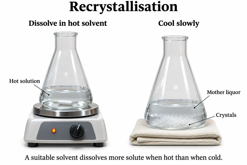
Realistic apparatus view
Purify a solid by dissolving it and allowing crystals to form during cooling.


Critical detail
Purify a solid by dissolving it and allowing crystals to form during cooling.
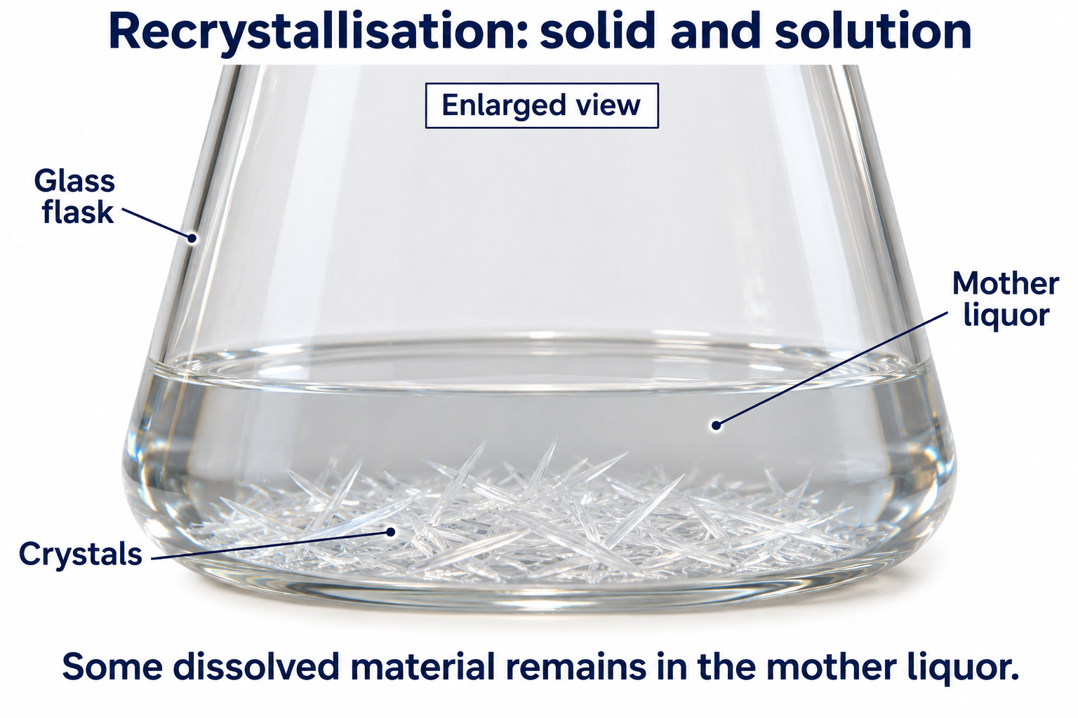
The needle-shaped crystals are generic; the white capsule represents a magnetic stir bar.
 CHEMISTRY · C10 · 3 VISUALSSeparating-funnel extractionSeparate immiscible liquid layers using a supported separating funnel.
Labelled schematic
Separate immiscible liquid layers using a supported separating funnel.


Realistic apparatus view
Separate immiscible liquid layers using a supported separating funnel.


Critical detail
Separate immiscible liquid layers using a supported separating funnel.
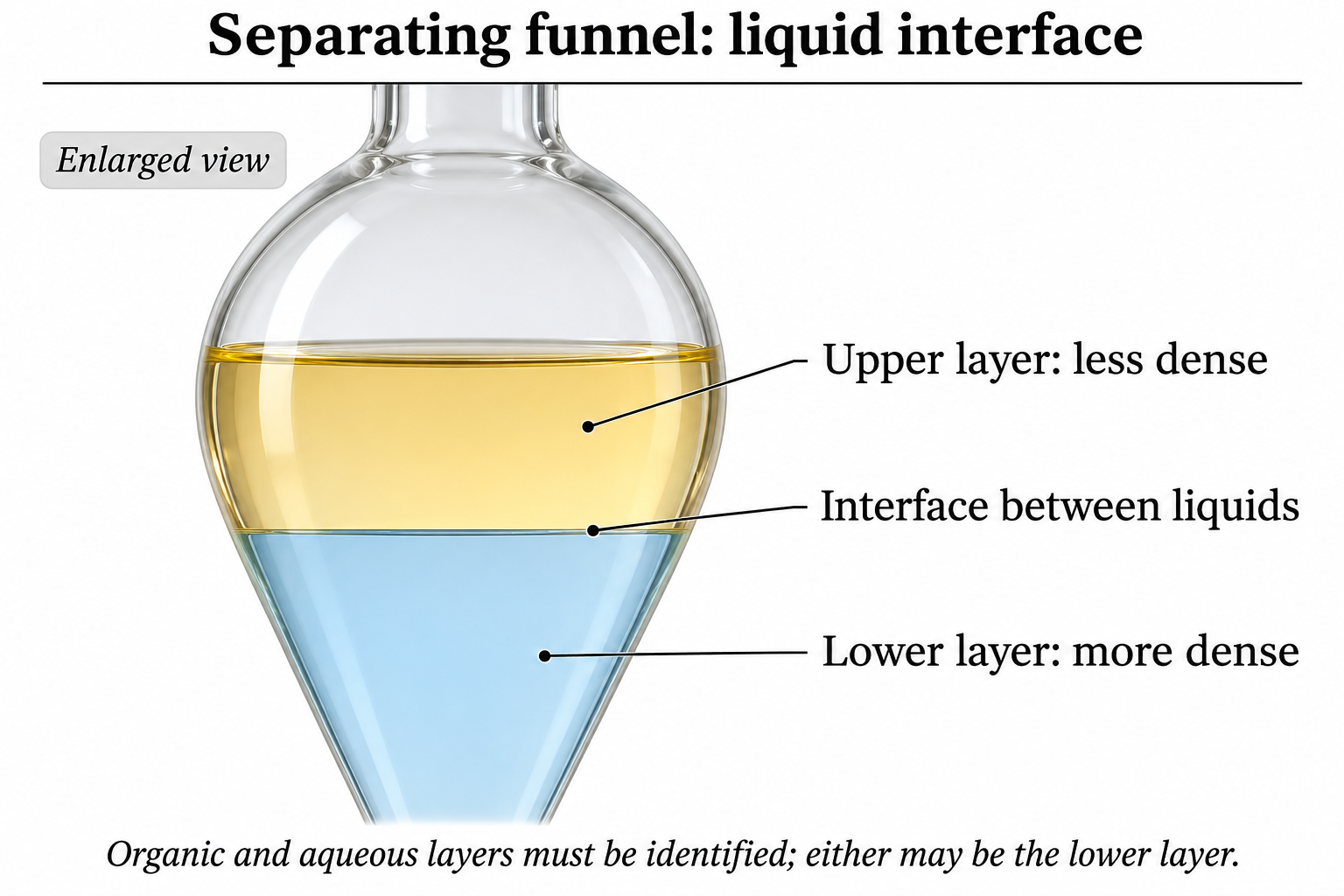
Layer colours are illustrative; chemical identity and density determine which actual liquid is on top.
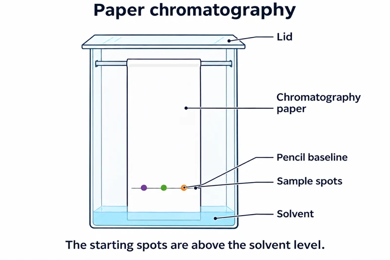 CHEMISTRY · C11 · 3 VISUALSPaper chromatographySeparate mixture components using paper and a developing solvent.
Labelled schematic
Separate mixture components using paper and a developing solvent.


Realistic apparatus view
Separate mixture components using paper and a developing solvent.

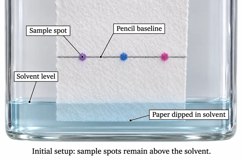
Critical detail
Separate mixture components using paper and a developing solvent.
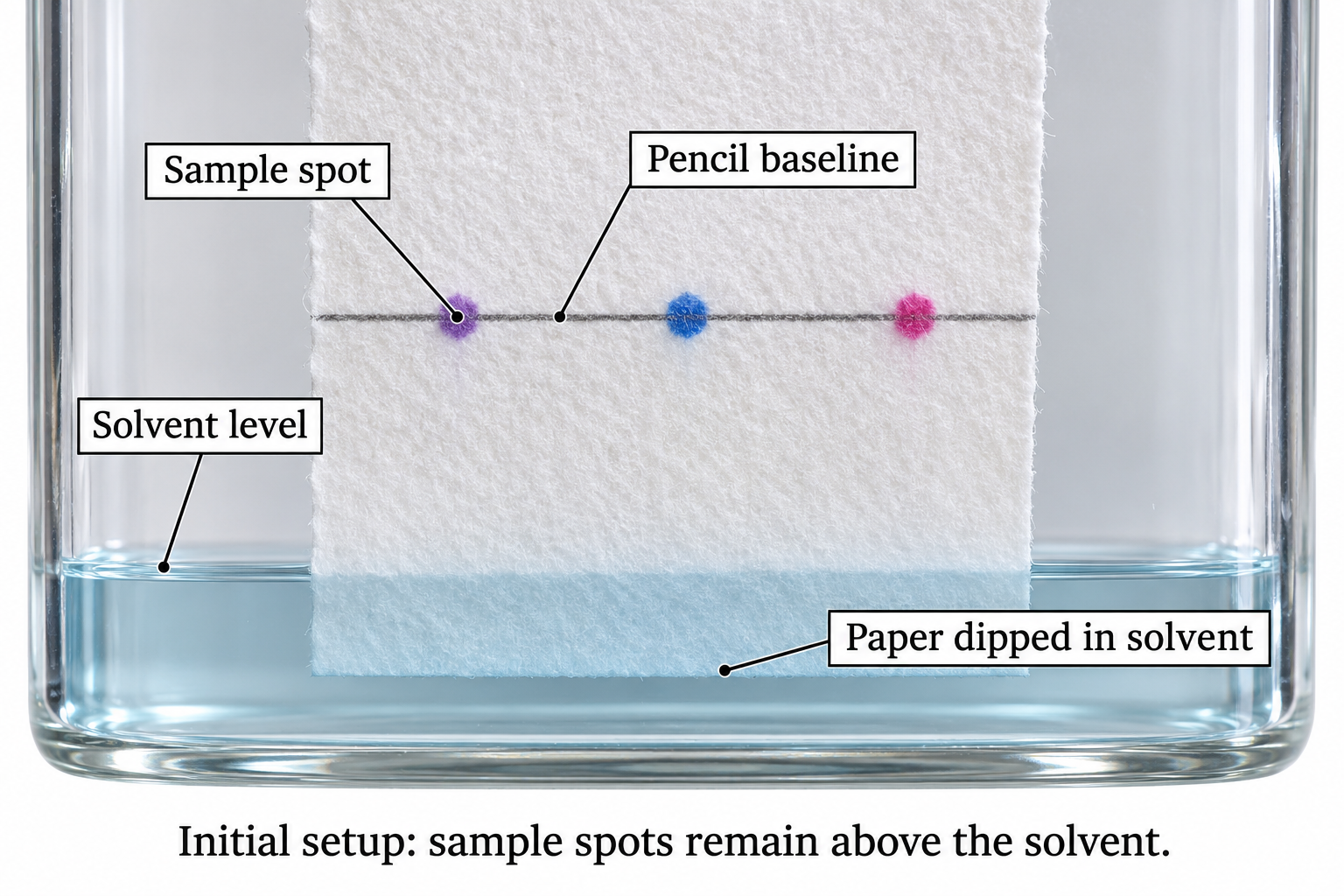
The images show the initial setup, with the sample above the solvent level.
 CHEMISTRY · C12 · 3 VISUALSThin-layer chromatographyDevelop a spotted TLC plate to compare mixture components.
Labelled schematic
Develop a spotted TLC plate to compare mixture components.


Realistic apparatus view
Develop a spotted TLC plate to compare mixture components.
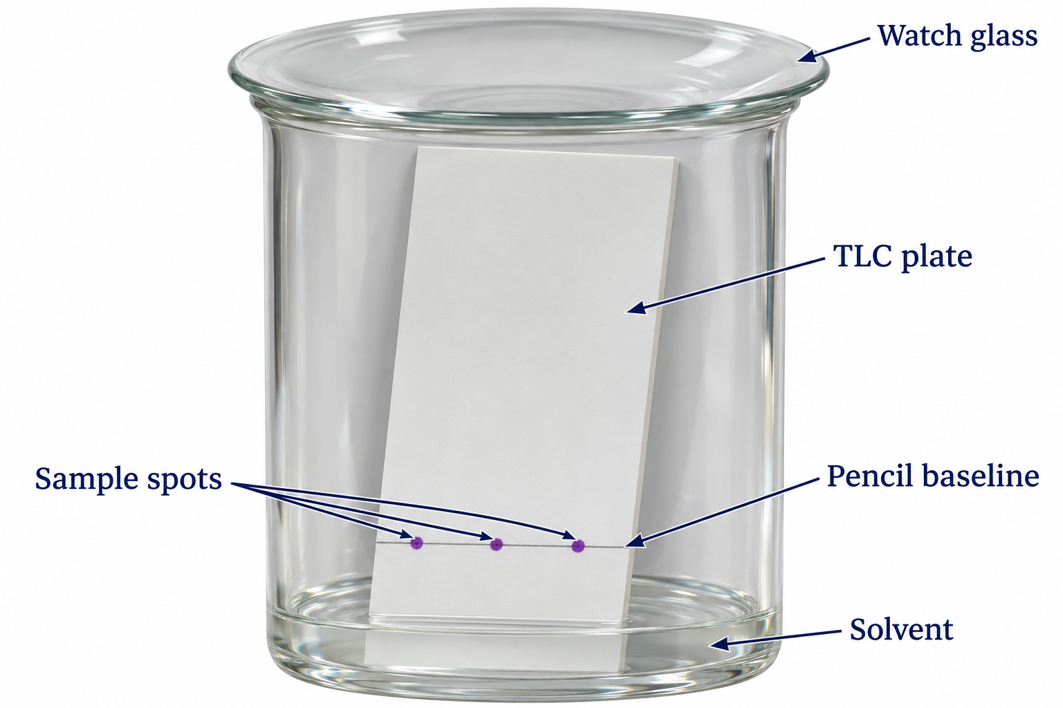

Critical detail
Develop a spotted TLC plate to compare mixture components.
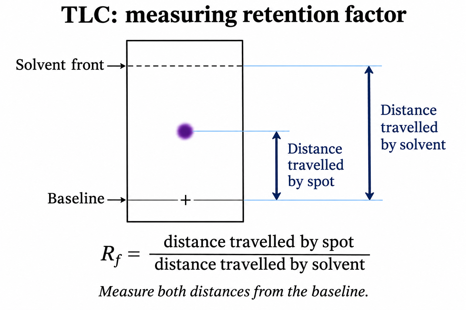
The detail illustrates Rf measurement; it is not a recorded chromatogram for a named substance.
 CHEMISTRY · C13 · 3 VISUALSGravity column chromatographySeparate mixture components as solvent moves through a packed column.
Labelled schematic
Separate mixture components as solvent moves through a packed column.
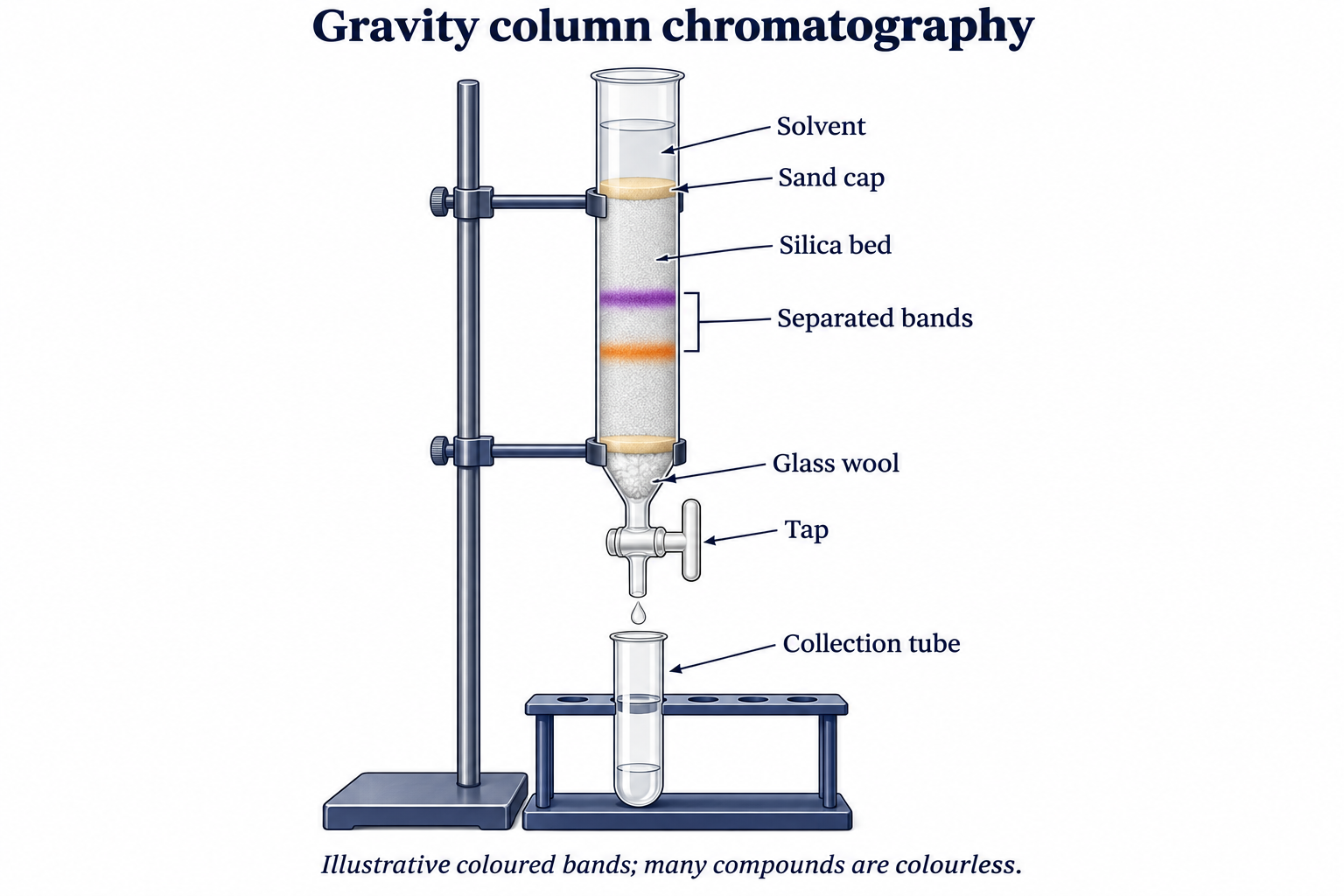

Realistic apparatus view
Separate mixture components as solvent moves through a packed column.
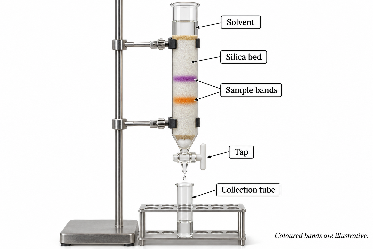

Critical detail
Separate mixture components as solvent moves through a packed column.

Bands and fractions illustrate the method, not measured retention or a specified chemical mixture.
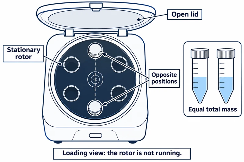 CHEMISTRY · C14 · 3 VISUALSCentrifugationSeparate suspended material by spinning balanced sample tubes.
Labelled schematic
Separate suspended material by spinning balanced sample tubes.
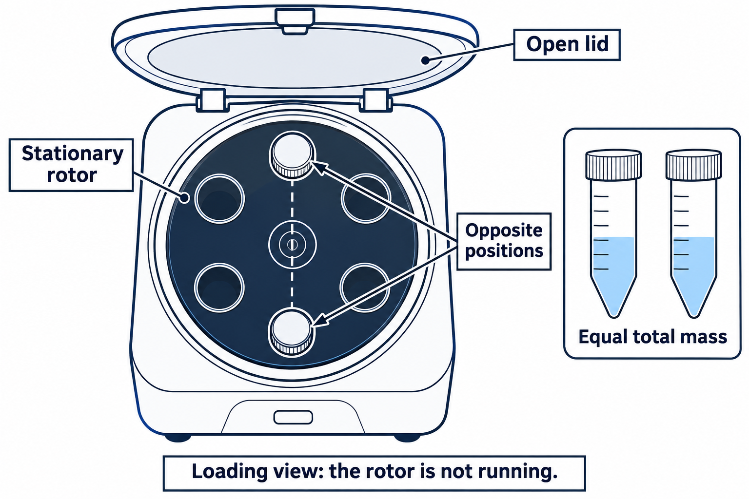

Realistic apparatus view
Separate suspended material by spinning balanced sample tubes.


Critical detail
Separate suspended material by spinning balanced sample tubes.

The images show a generic balanced arrangement, not a prescribed speed or run time.
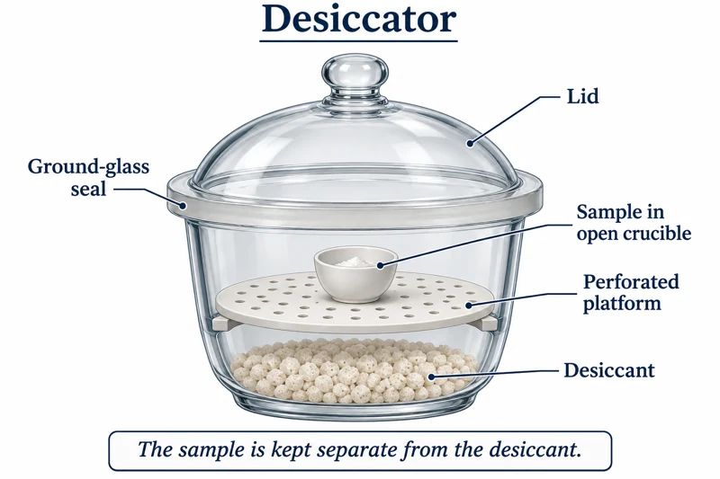 CHEMISTRY · C15 · 3 VISUALSDrying and desiccator storageKeep a prepared sample in a dry enclosure above a desiccant.
Labelled schematic
Keep a prepared sample in a dry enclosure above a desiccant.
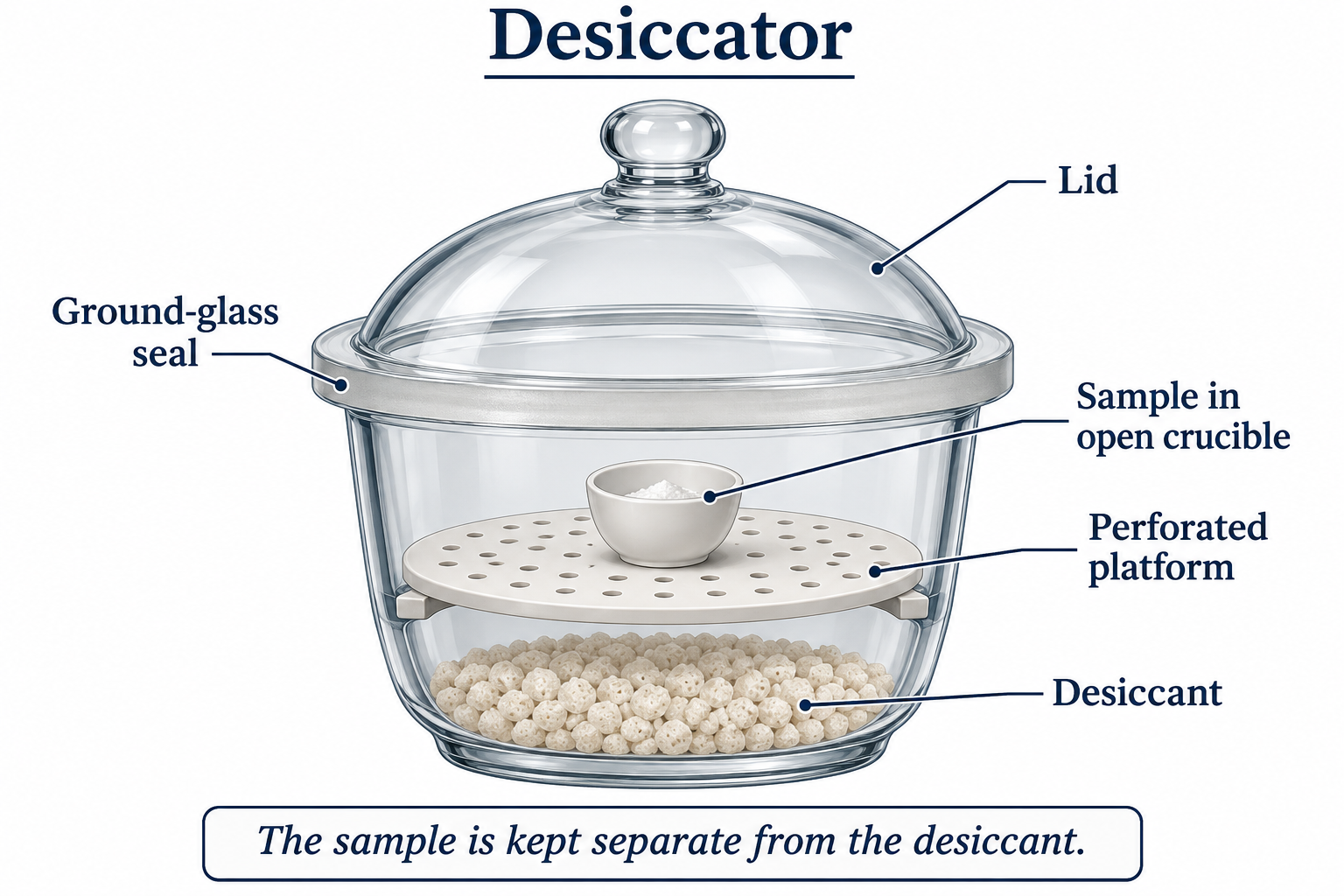

Realistic apparatus view
Keep a prepared sample in a dry enclosure above a desiccant.
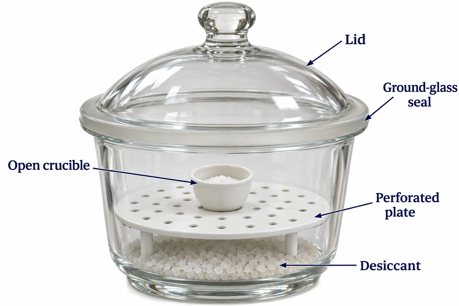
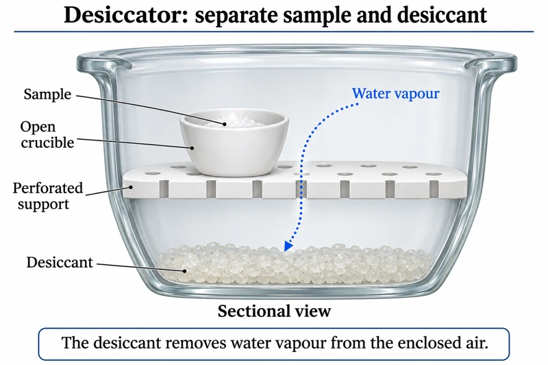
Critical detail
Keep a prepared sample in a dry enclosure above a desiccant.
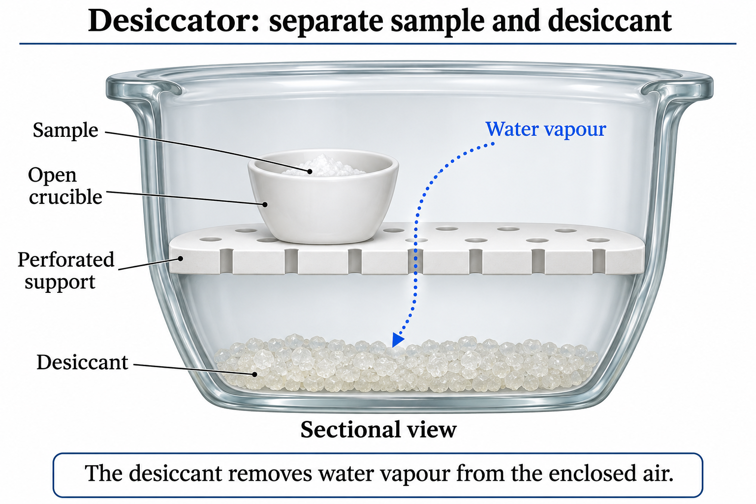
The detail is a section with the lid omitted for visibility, not the storage position.
 CHEMISTRY · C16 · 3 VISUALSStandard-solution preparationTransfer a known amount of solute into a volumetric flask and dilute to a defined volume.
Labelled schematic
Transfer a known amount of solute into a volumetric flask and dilute to a defined volume.
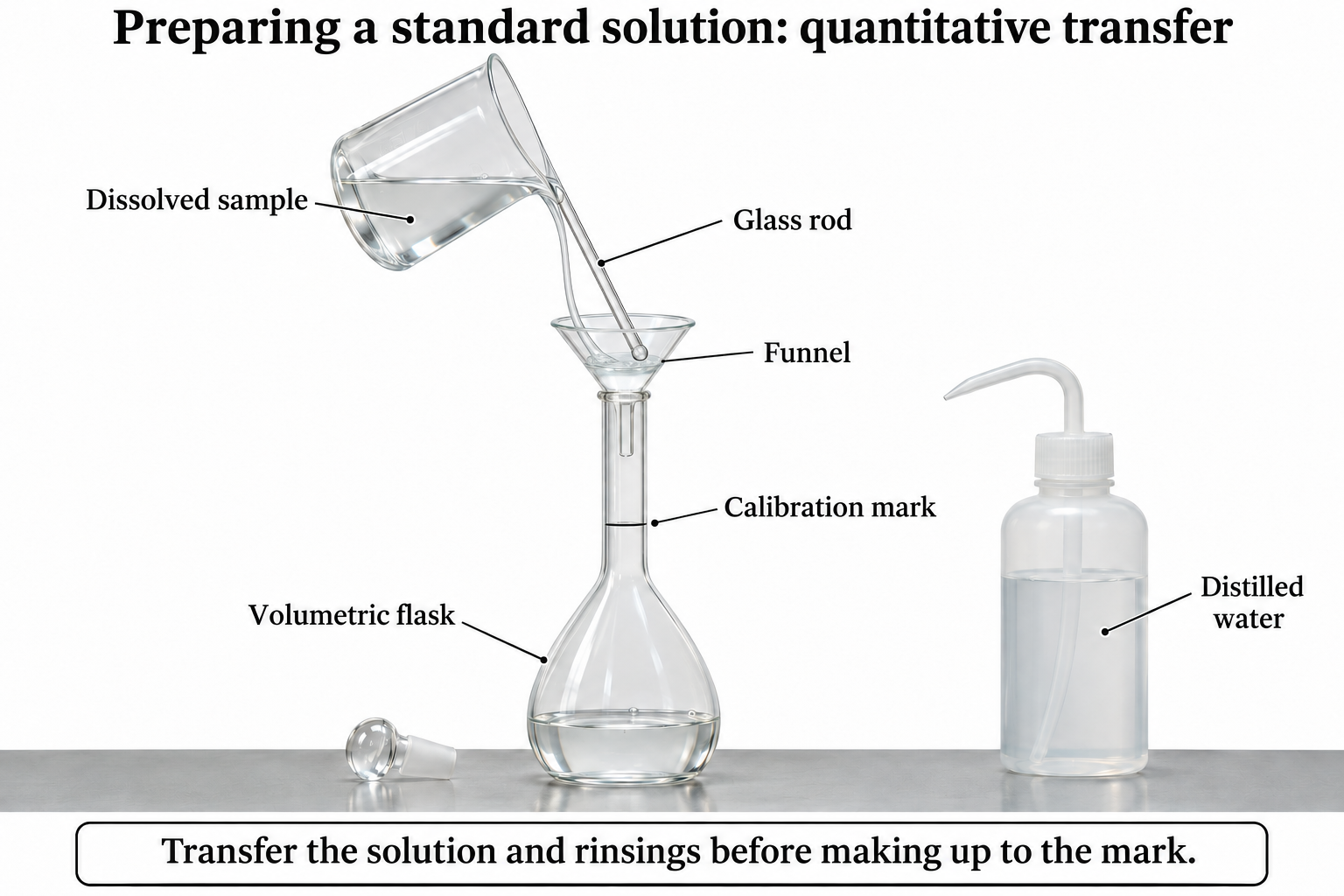

Realistic apparatus view
Transfer a known amount of solute into a volumetric flask and dilute to a defined volume.


Critical detail
Transfer a known amount of solute into a volumetric flask and dilute to a defined volume.

An accurately weighed known solute is a prerequisite; the artwork is not a volumetric calibration.
 CHEMISTRY · C17 · 3 VISUALSVolumetric transfer and dilutionUse a volumetric pipette to transfer an aliquot for accurate dilution.
Labelled schematic
Use a volumetric pipette to transfer an aliquot for accurate dilution.


Realistic apparatus view
Use a volumetric pipette to transfer an aliquot for accurate dilution.
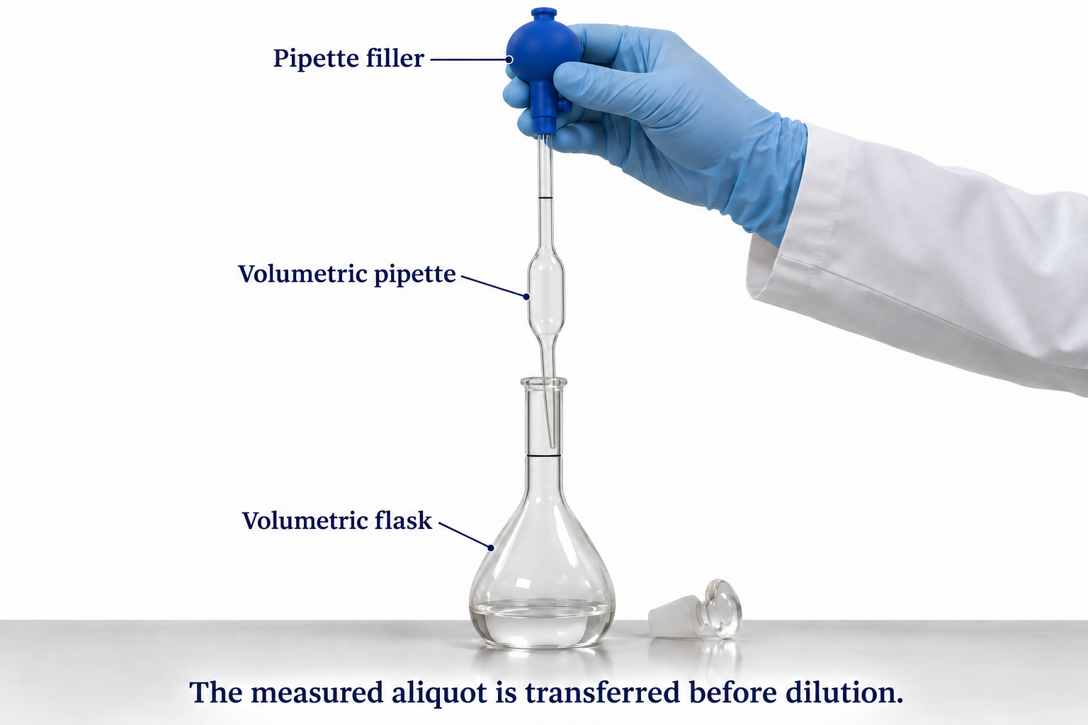

Critical detail
Use a volumetric pipette to transfer an aliquot for accurate dilution.

The delivery detail illustrates tip contact and residual liquid for the depicted pipette, not a universal blow-out instruction.
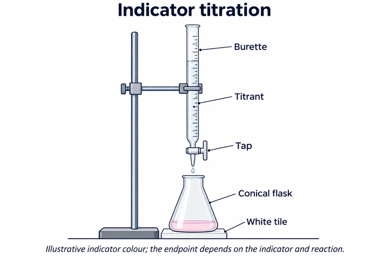 CHEMISTRY · C18 · 3 VISUALSIndicator titrationMeasure the volume of titrant needed to reach an indicator endpoint.
Labelled schematic
Measure the volume of titrant needed to reach an indicator endpoint.


Realistic apparatus view
Measure the volume of titrant needed to reach an indicator endpoint.


Critical detail
Measure the volume of titrant needed to reach an indicator endpoint.

Colour and burette ticks are illustrative rather than an endpoint determination or reading exercise.
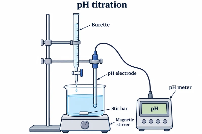 CHEMISTRY · C19 · 3 VISUALSpH titrationRecord pH as titrant is added to a stirred solution.
Labelled schematic
Record pH as titrant is added to a stirred solution.


Realistic apparatus view
Record pH as titrant is added to a stirred solution.


Critical detail
Record pH as titrant is added to a stirred solution.
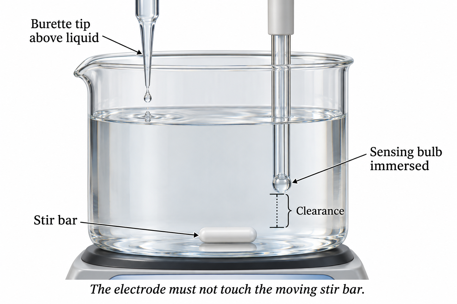
The probe is generic; no manufacturer-specific internal construction or measured titration curve is claimed.
 CHEMISTRY · C20 · 3 VISUALSConductometric titrationFollow conductivity as titrant is added to a stirred solution.
Labelled schematic
Follow conductivity as titrant is added to a stirred solution.
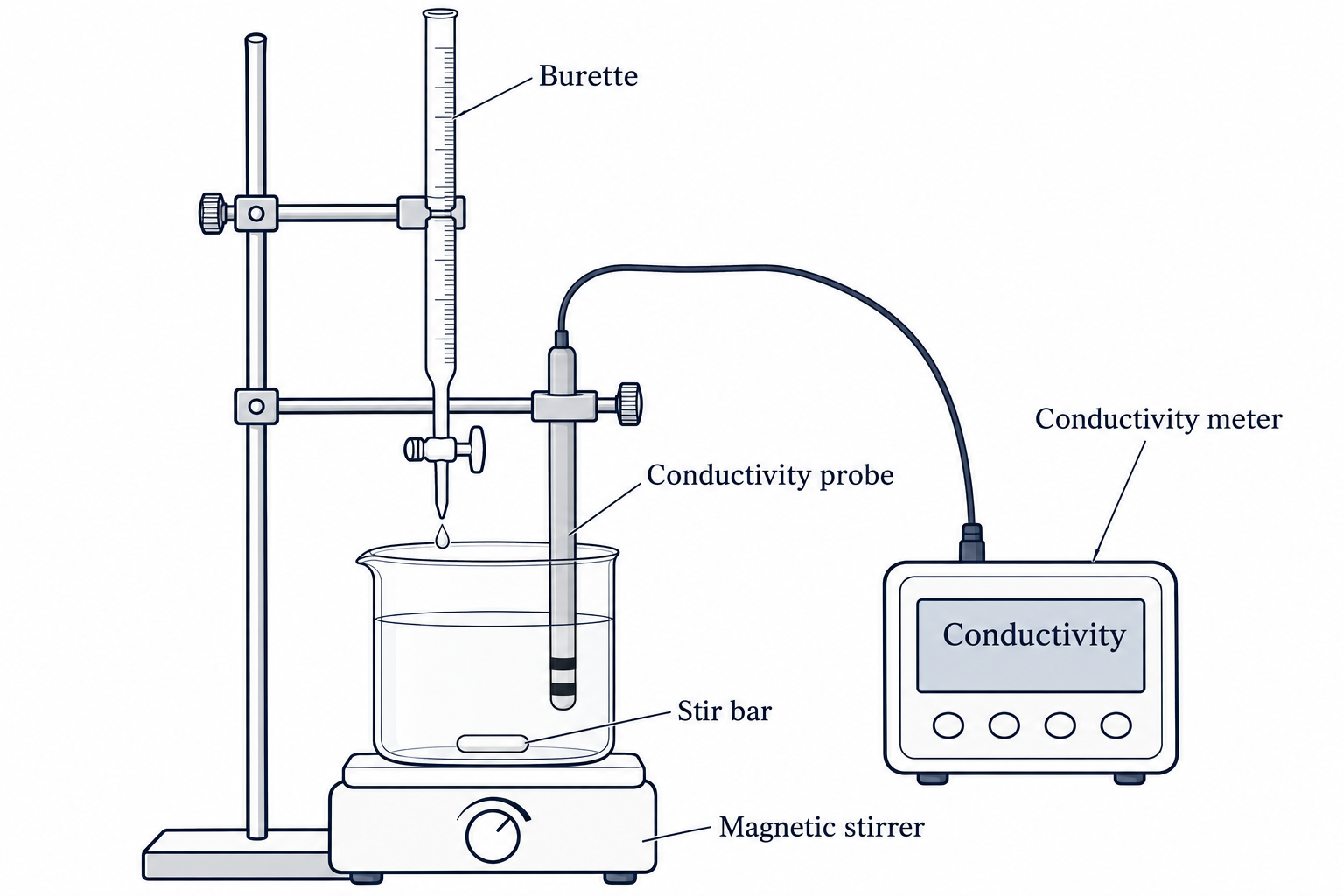

Realistic apparatus view
Follow conductivity as titrant is added to a stirred solution.


Critical detail
Follow conductivity as titrant is added to a stirred solution.

The two-ring probe is a simplified instrument representation, not a specified cell constant.
 CHEMISTRY · C21 · 3 VISUALSColorimetryUse cuvettes and an optical instrument to compare solution absorbance.
Labelled schematic
Use cuvettes and an optical instrument to compare solution absorbance.


Realistic apparatus view
Use cuvettes and an optical instrument to compare solution absorbance.

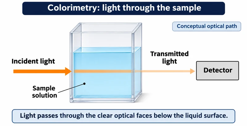
Critical detail
Use cuvettes and an optical instrument to compare solution absorbance.

The images show a generic loading arrangement and conceptual optical path, not a specific spectrophotometer design.
 CHEMISTRY · C22 · 3 VISUALSGravimetric precipitation analysisCollect and weigh a precipitate to relate its mass to the amount of analyte.
Labelled schematic
Collect and weigh a precipitate to relate its mass to the amount of analyte.
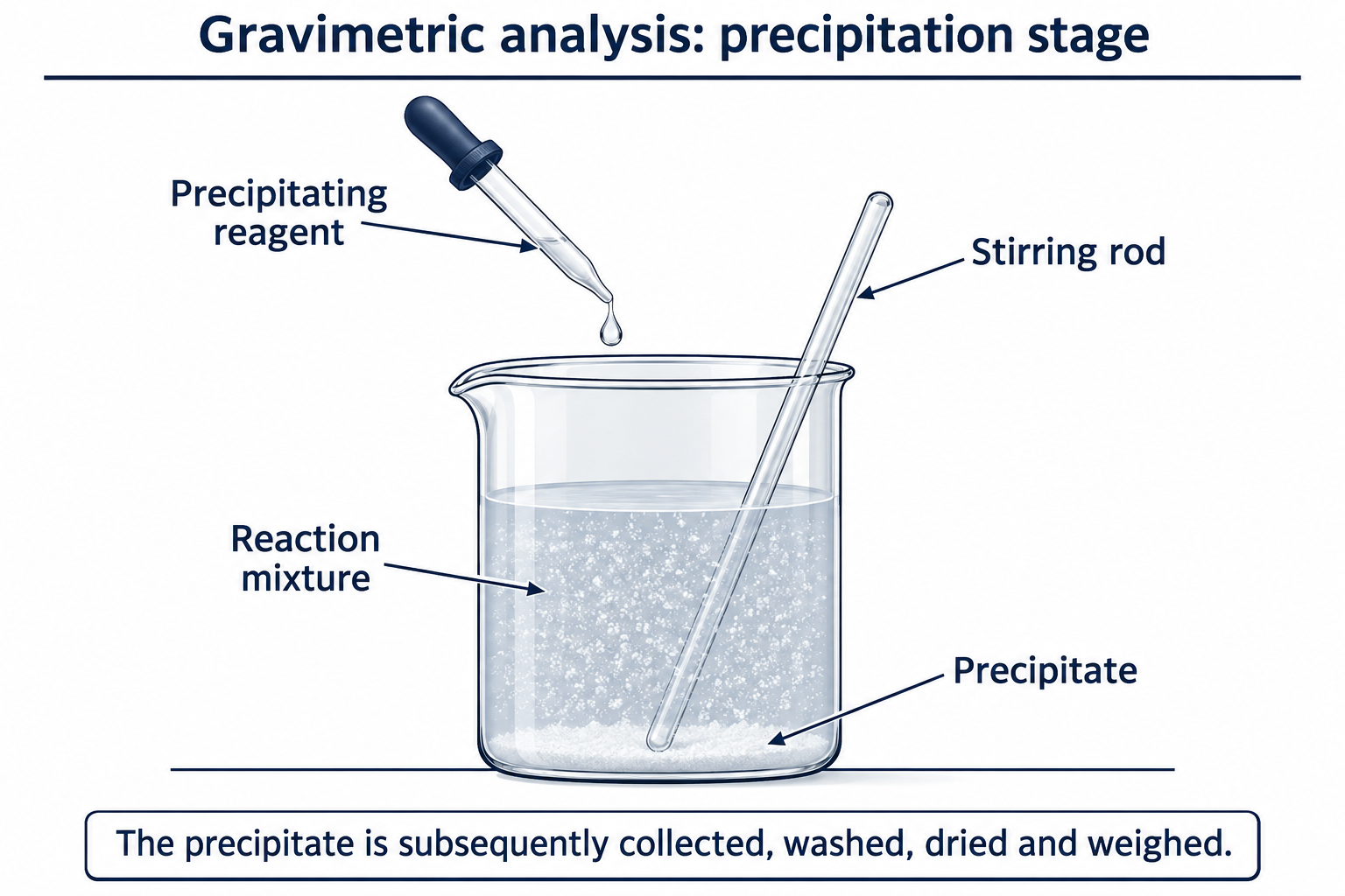

Realistic apparatus view
Collect and weigh a precipitate to relate its mass to the amount of analyte.
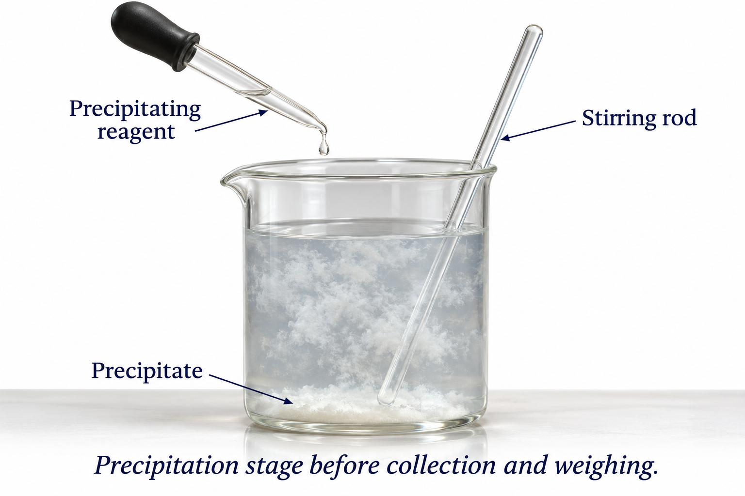

Critical detail
Collect and weigh a precipitate to relate its mass to the amount of analyte.
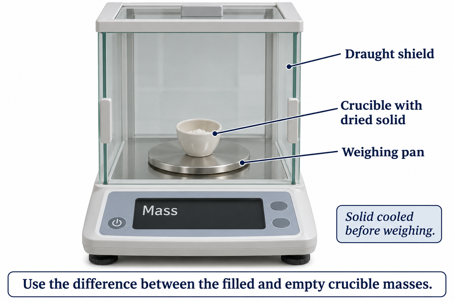
A quantitative result requires suitable preparation and drying to constant mass, not merely weighing a wet precipitate.
 CHEMISTRY · C23 · 3 VISUALSMelting-point determinationObserve a small capillary sample while measuring its melting range.
Labelled schematic
Observe a small capillary sample while measuring its melting range.
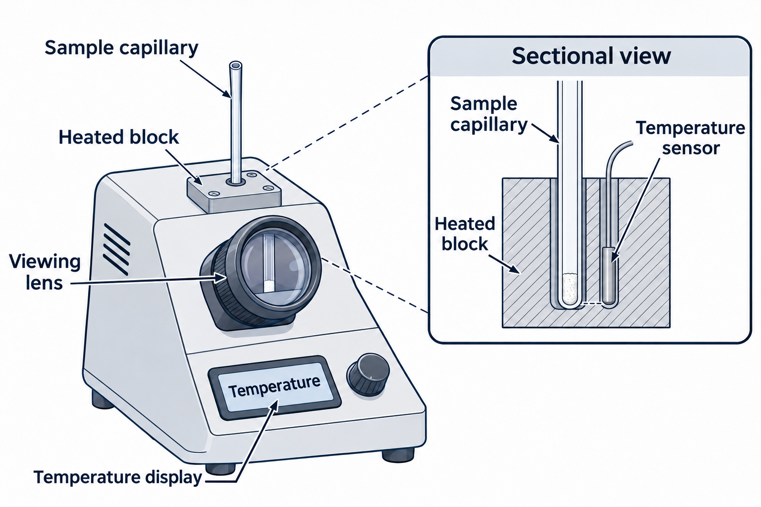

Realistic apparatus view
Observe a small capillary sample while measuring its melting range.


Critical detail
Observe a small capillary sample while measuring its melting range.
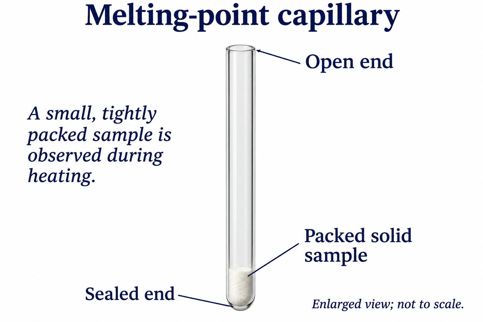
The instrument and sample are illustrative rather than a substance identification or measured melting range.
 CHEMISTRY · C24 · 3 VISUALSBoiling temperature of waterMeasure water temperature during boiling using a heated vessel and thermometer.
Labelled schematic
Measure water temperature during boiling using a heated vessel and thermometer.
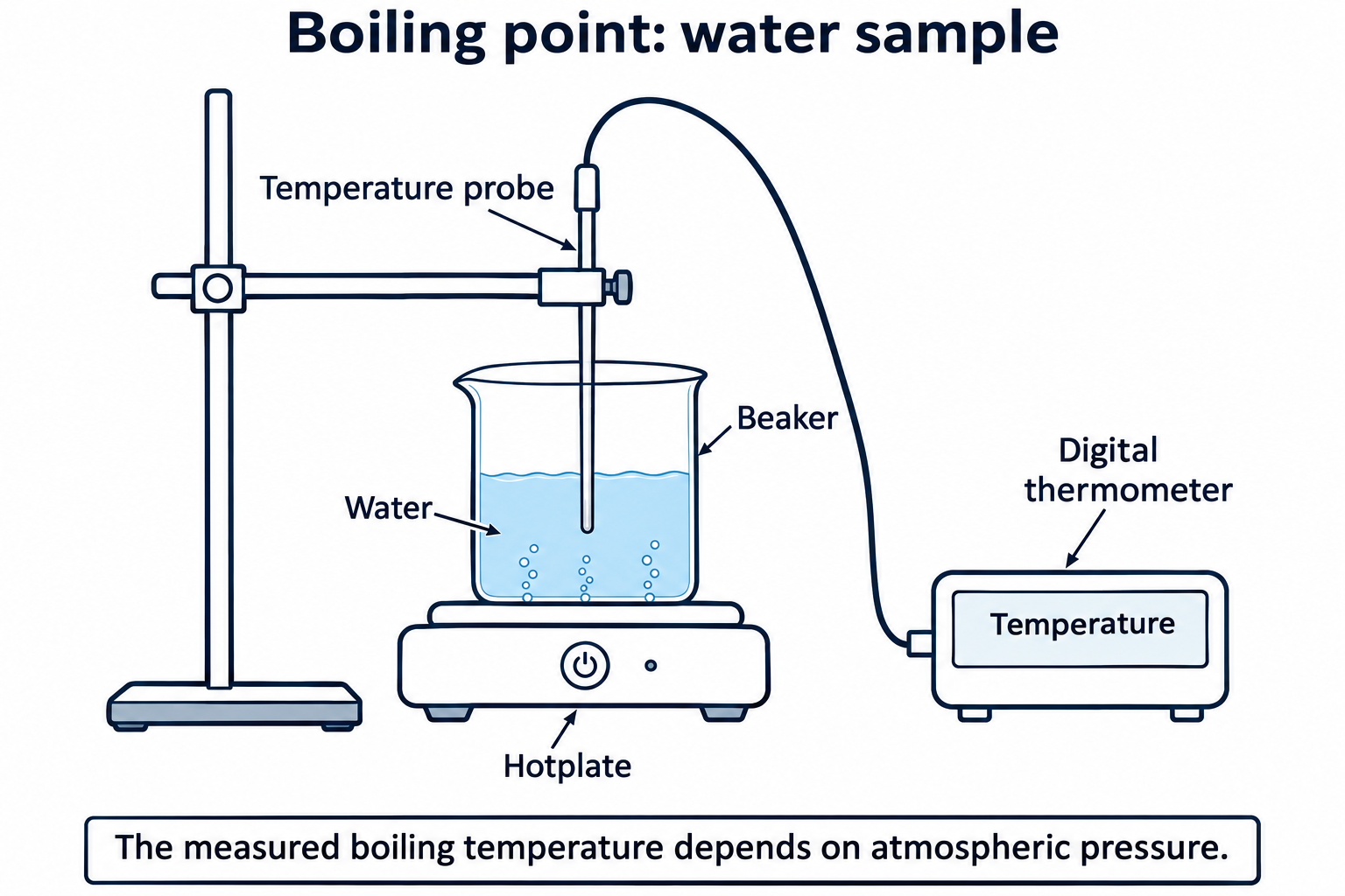

Realistic apparatus view
Measure water temperature during boiling using a heated vessel and thermometer.


Critical detail
Measure water temperature during boiling using a heated vessel and thermometer.

This set depicts water, not a general small-scale method for volatile organic liquids; boiling temperature depends on pressure.
 CHEMISTRY · C25 · 3 VISUALSInsulated-cup calorimetryMeasure temperature change in an insulated cup to estimate heat transfer during a reaction.
Labelled schematic
Measure temperature change in an insulated cup to estimate heat transfer during a reaction.


Realistic apparatus view
Measure temperature change in an insulated cup to estimate heat transfer during a reaction.
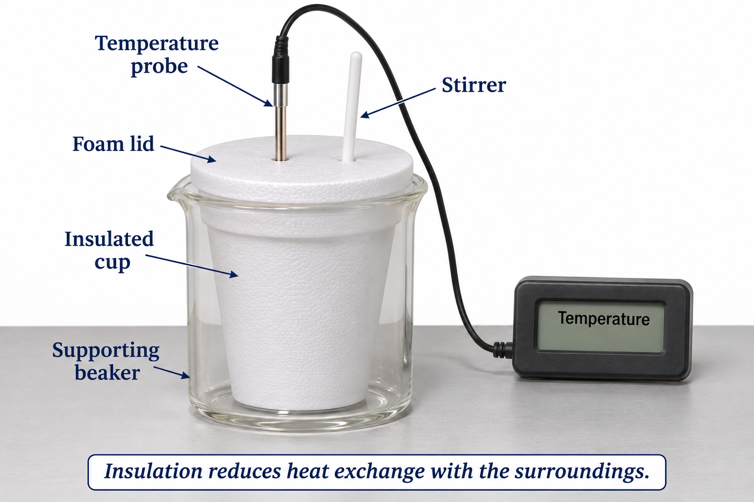

Critical detail
Measure temperature change in an insulated cup to estimate heat transfer during a reaction.

Heat exchange with the surroundings and the apparatus can affect the estimate.
 CHEMISTRY · C26 · 3 VISUALSCombustion calorimetryUse a burning fuel to heat water and estimate transferred energy.
Labelled schematic
Use a burning fuel to heat water and estimate transferred energy.
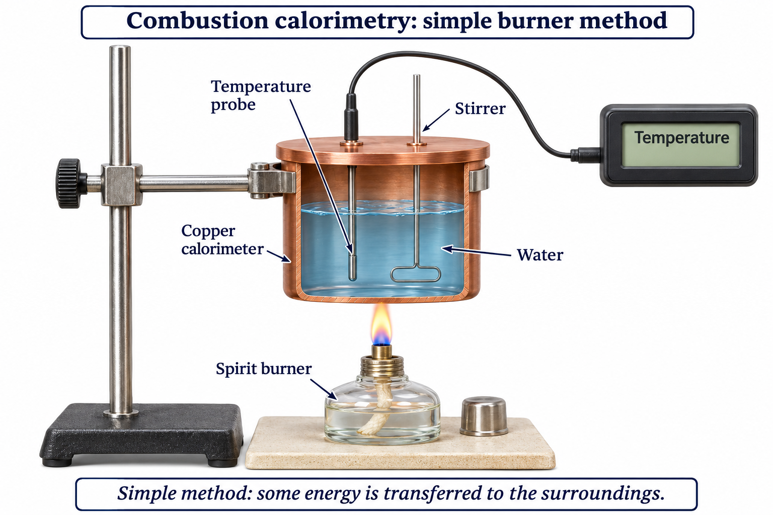

Realistic apparatus view
Use a burning fuel to heat water and estimate transferred energy.
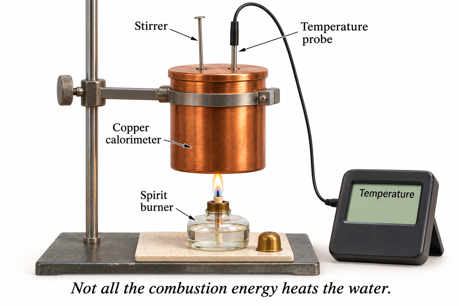

Critical detail
Use a burning fuel to heat water and estimate transferred energy.
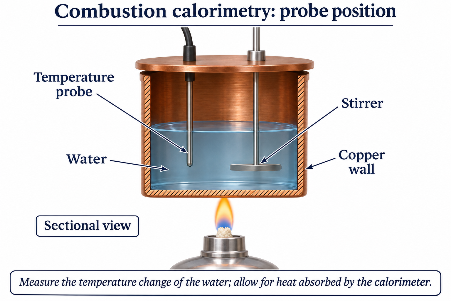
The apparatus measures energy reaching the water; heat loss and incomplete combustion can affect results.
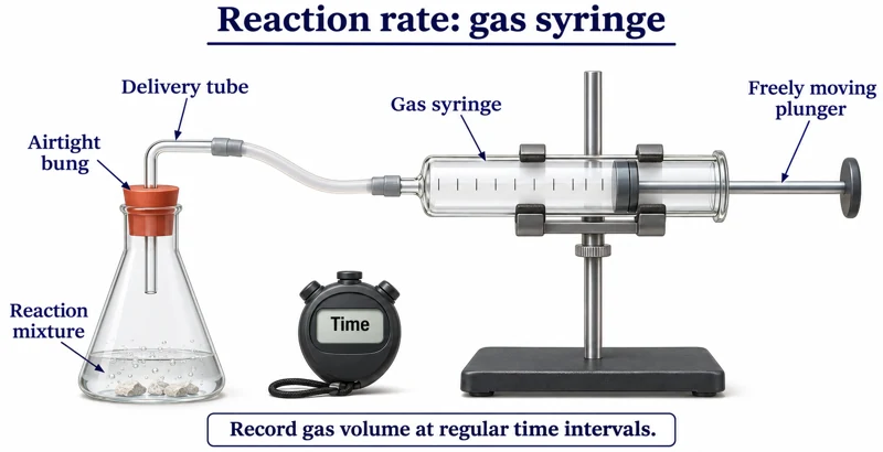 CHEMISTRY · C27 · 3 VISUALSGas-syringe reaction ratesFollow gas volume over time as a reaction proceeds.
Labelled schematic
Follow gas volume over time as a reaction proceeds.


Realistic apparatus view
Follow gas volume over time as a reaction proceeds.

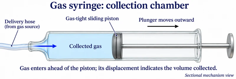
Critical detail
Follow gas volume over time as a reaction proceeds.

The syringe and piston arrangement is illustrative and supplies no calibrated reaction-rate data.
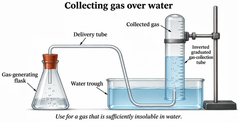 CHEMISTRY · C28 · 3 VISUALSGas collection over waterCollect a suitable gas in an inverted water-filled graduated tube.
Labelled schematic
Collect a suitable gas in an inverted water-filled graduated tube.
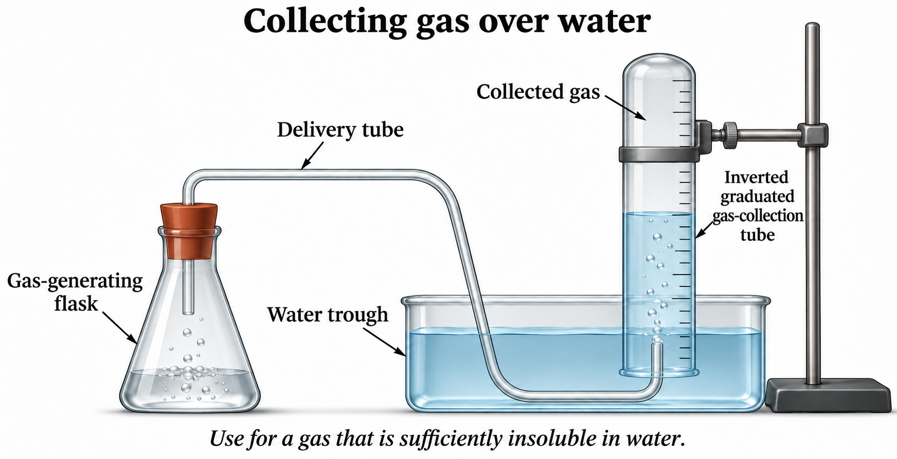

Realistic apparatus view
Collect a suitable gas in an inverted water-filled graduated tube.


Critical detail
Collect a suitable gas in an inverted water-filled graduated tube.

The gas must not react appreciably with or dissolve in water; unequal water levels mean the gas pressure is not simply atmospheric.
 CHEMISTRY · C29 · 3 VISUALSMass-loss reaction ratesUse a balance to follow mass loss as gas escapes from a reaction vessel.
Labelled schematic
Use a balance to follow mass loss as gas escapes from a reaction vessel.
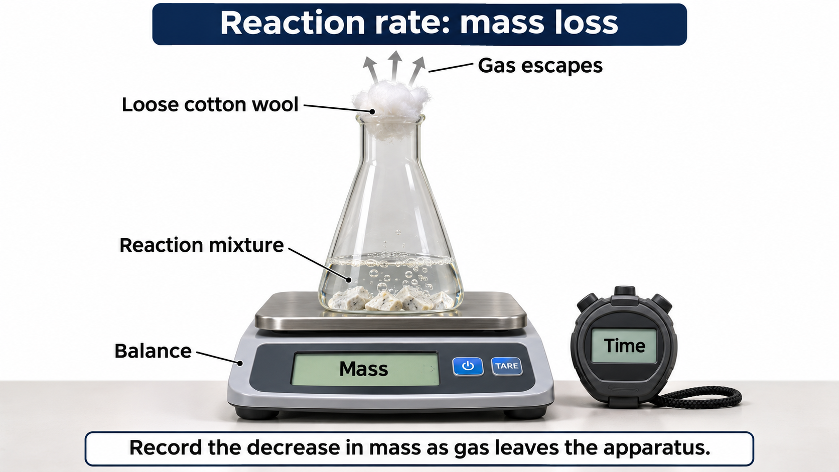

Realistic apparatus view
Use a balance to follow mass loss as gas escapes from a reaction vessel.


Critical detail
Use a balance to follow mass loss as gas escapes from a reaction vessel.
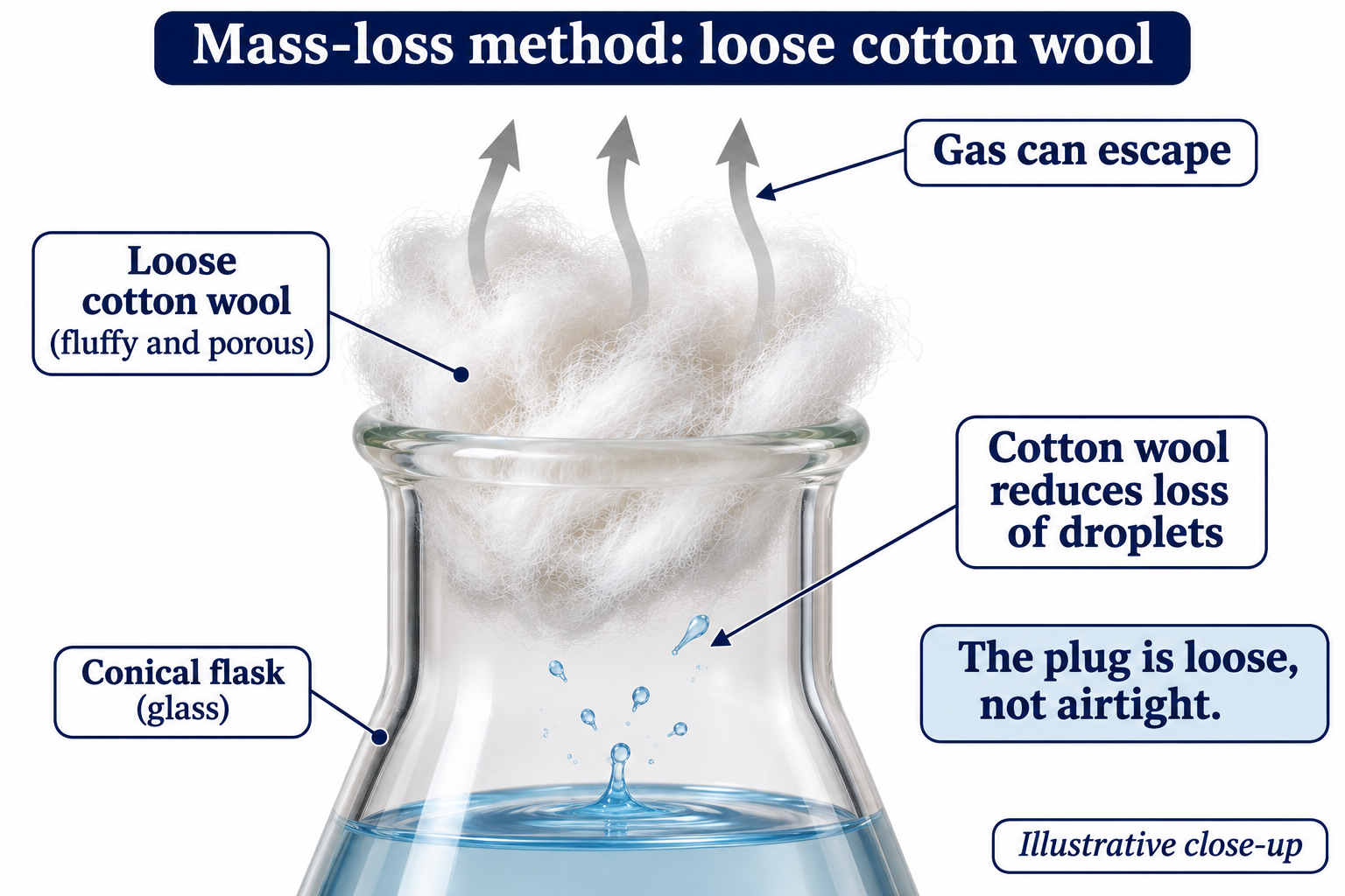
Other mass losses, such as evaporation or splashing, would also affect the reading.
 CHEMISTRY · C30 · 3 VISUALSClock reactionCompare the time taken for a reaction mixture to develop a visible endpoint.
Labelled schematic
Compare the time taken for a reaction mixture to develop a visible endpoint.


Realistic apparatus view
Compare the time taken for a reaction mixture to develop a visible endpoint.
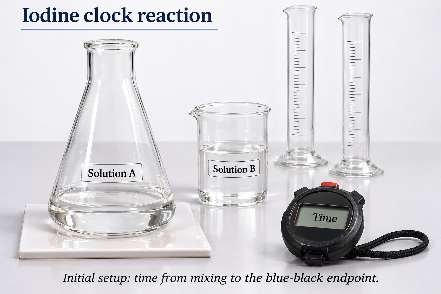

Critical detail
Compare the time taken for a reaction mixture to develop a visible endpoint.

The delayed blue-black change is illustrative; in the depicted iodine-clock principle the reducing agent is depleted before the colour persists.
 CHEMISTRY · C31 · 3 VISUALSDisappearing-cross reactionFollow increasing cloudiness by timing when a cross beneath the reaction vessel is obscured.
Labelled schematic
Follow increasing cloudiness by timing when a cross beneath the reaction vessel is obscured.


Realistic apparatus view
Follow increasing cloudiness by timing when a cross beneath the reaction vessel is obscured.
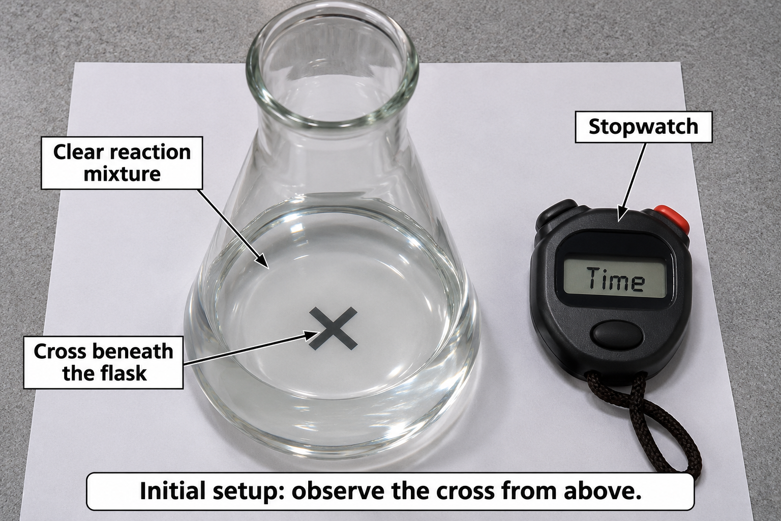

Critical detail
Follow increasing cloudiness by timing when a cross beneath the reaction vessel is obscured.
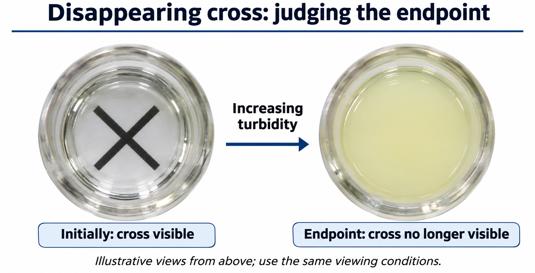
The visual endpoint depends on observation conditions and is not a continuous concentration measurement.
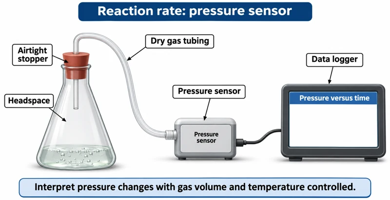 CHEMISTRY · C32 · 3 VISUALSPressure-sensor reaction ratesRecord pressure changes as gas is produced in a reaction vessel.
Labelled schematic
Record pressure changes as gas is produced in a reaction vessel.


Realistic apparatus view
Record pressure changes as gas is produced in a reaction vessel.
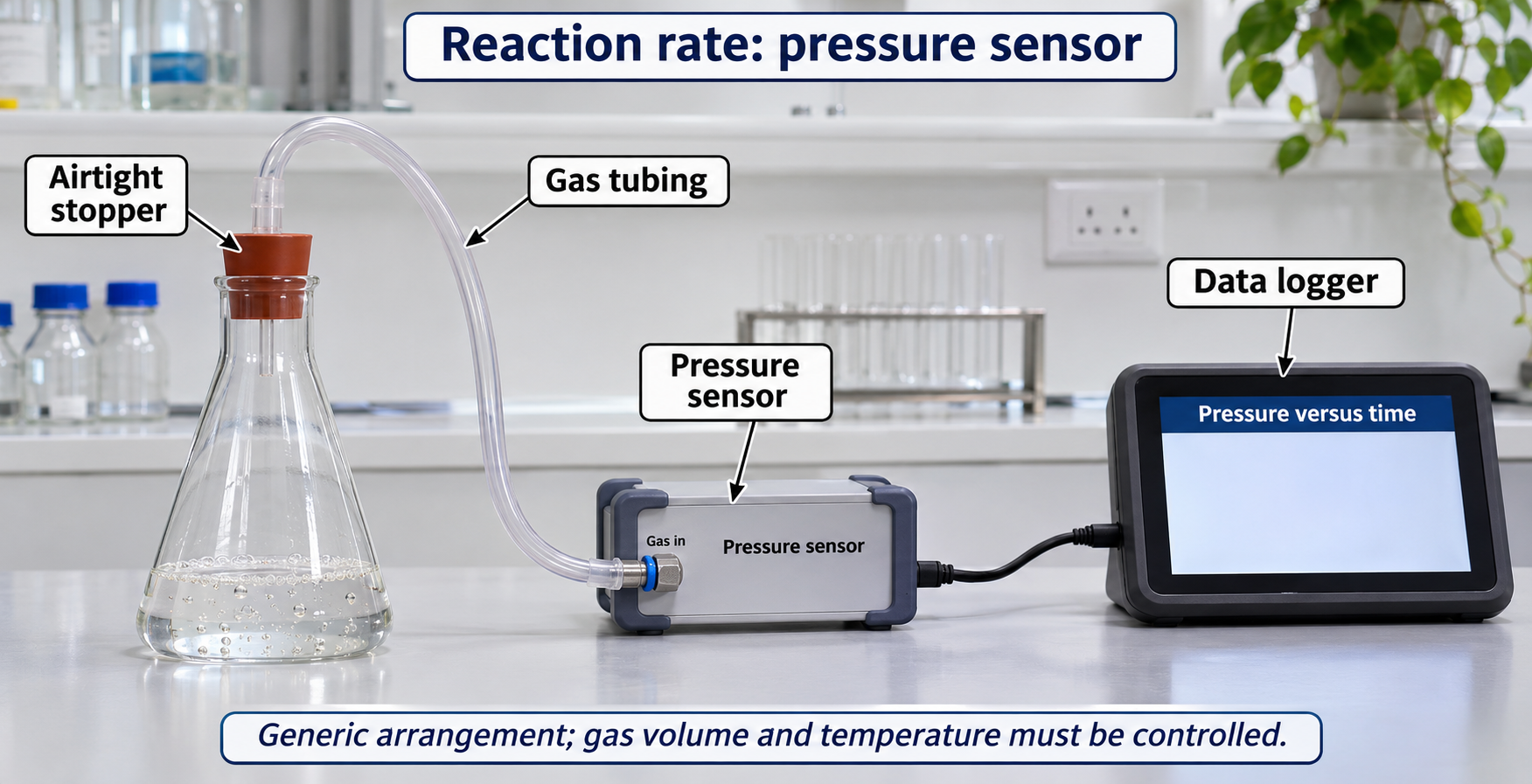
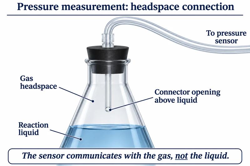
Critical detail
Record pressure changes as gas is produced in a reaction vessel.
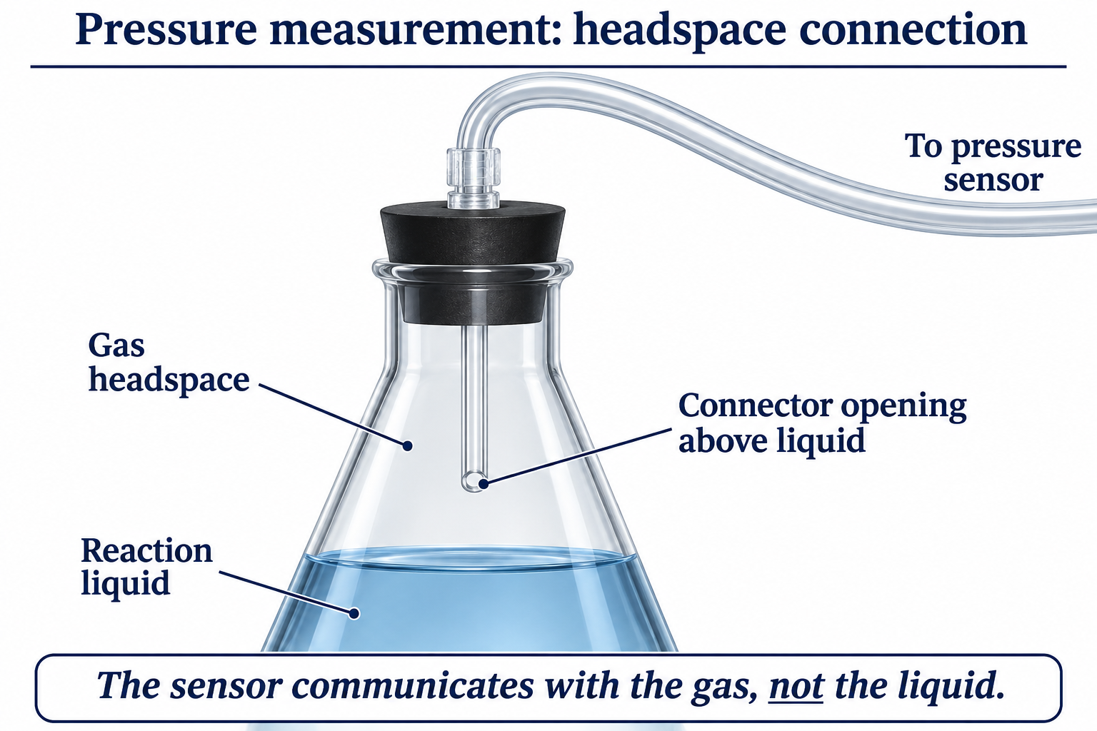
Pressure also depends on gas volume and temperature; the sensor depiction is generic.
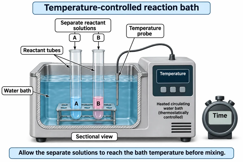 CHEMISTRY · C33 · 3 VISUALSTemperature-controlled kinetics bathEquilibrate reaction solutions in a water bath before comparing reaction rates.
Labelled schematic
Equilibrate reaction solutions in a water bath before comparing reaction rates.


Realistic apparatus view
Equilibrate reaction solutions in a water bath before comparing reaction rates.
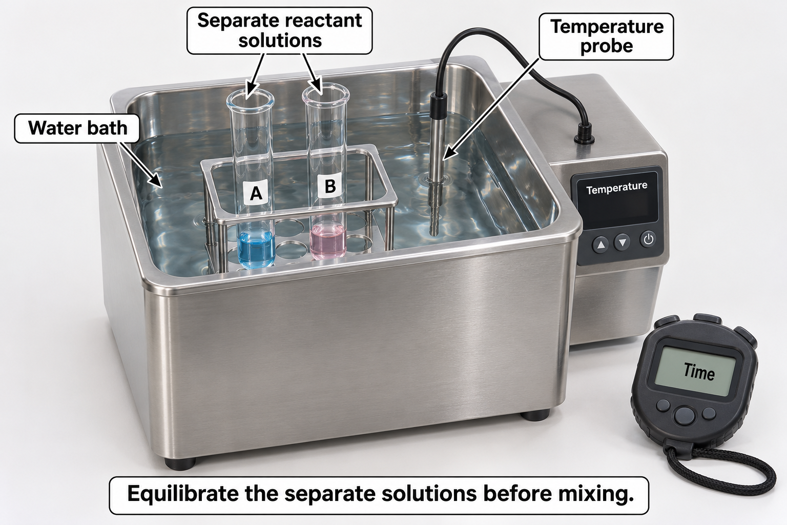

Critical detail
Equilibrate reaction solutions in a water bath before comparing reaction rates.
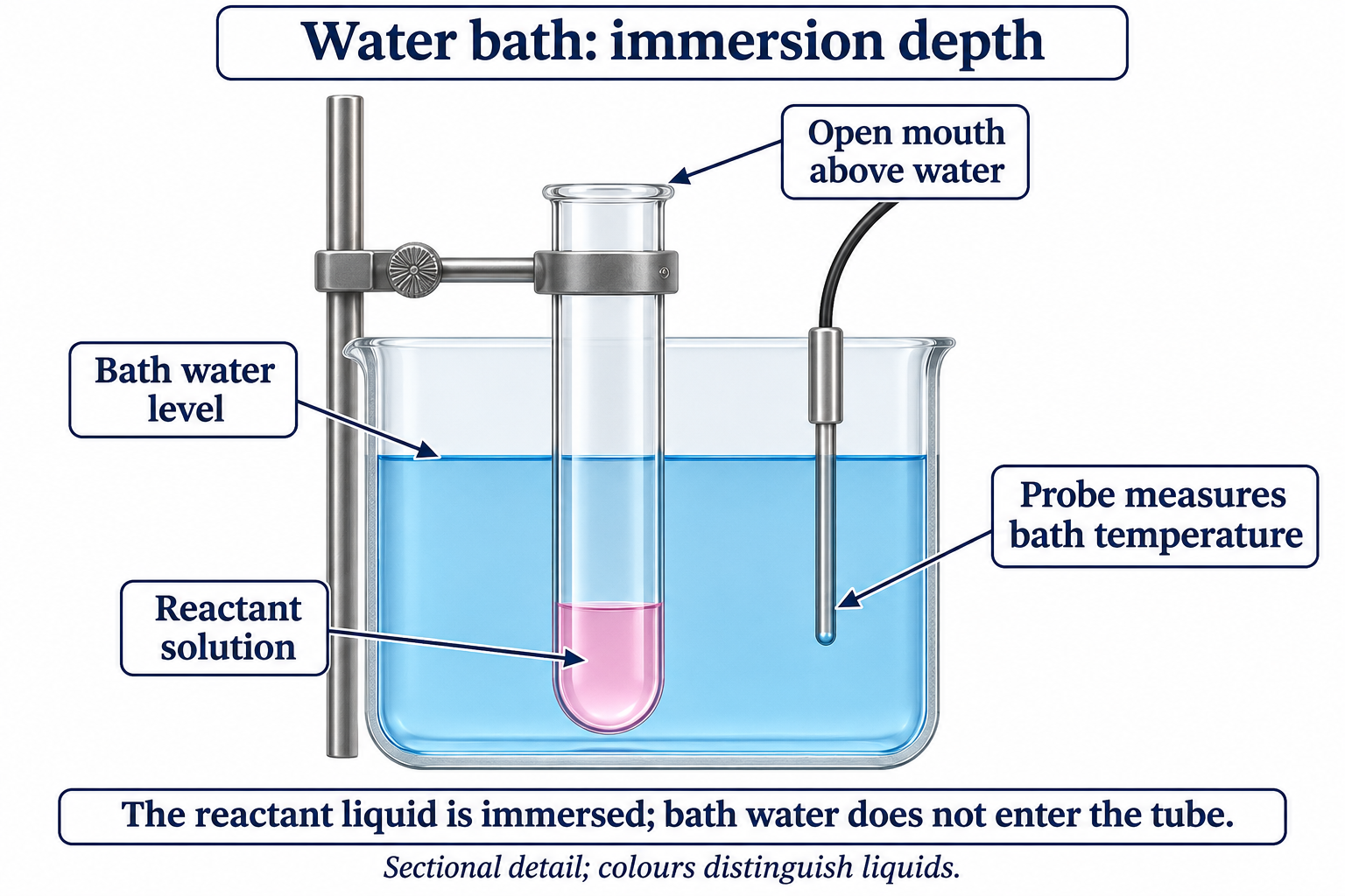
Separate solutions are brought to the chosen temperature before mixing; colours do not identify reagents.
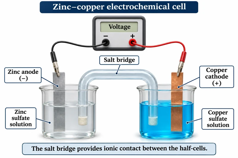 CHEMISTRY · C34 · 3 VISUALSElectrochemical cellMeasure potential difference between two half-cells connected by a salt bridge.
Labelled schematic
Measure potential difference between two half-cells connected by a salt bridge.
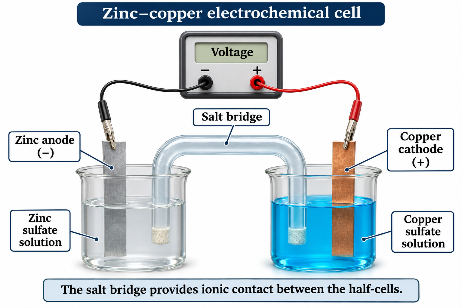
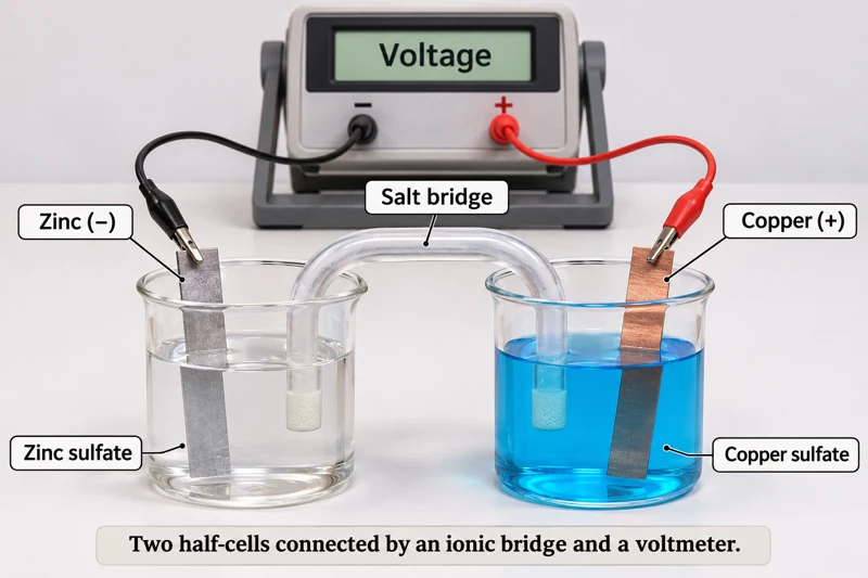
Realistic apparatus view
Measure potential difference between two half-cells connected by a salt bridge.
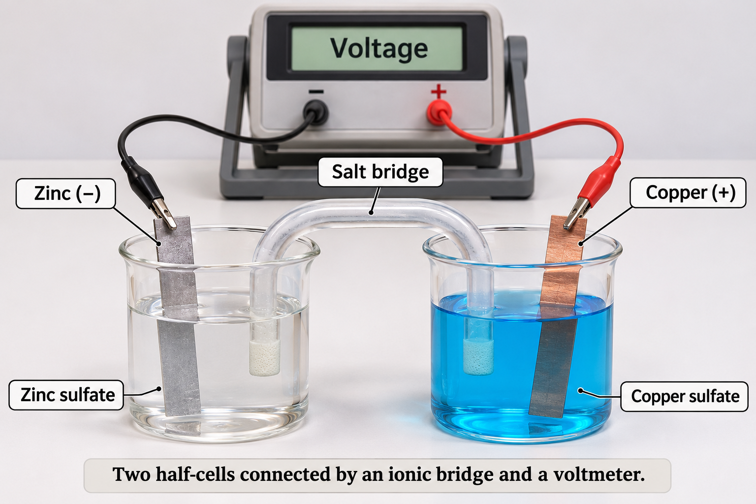

Critical detail
Measure potential difference between two half-cells connected by a salt bridge.
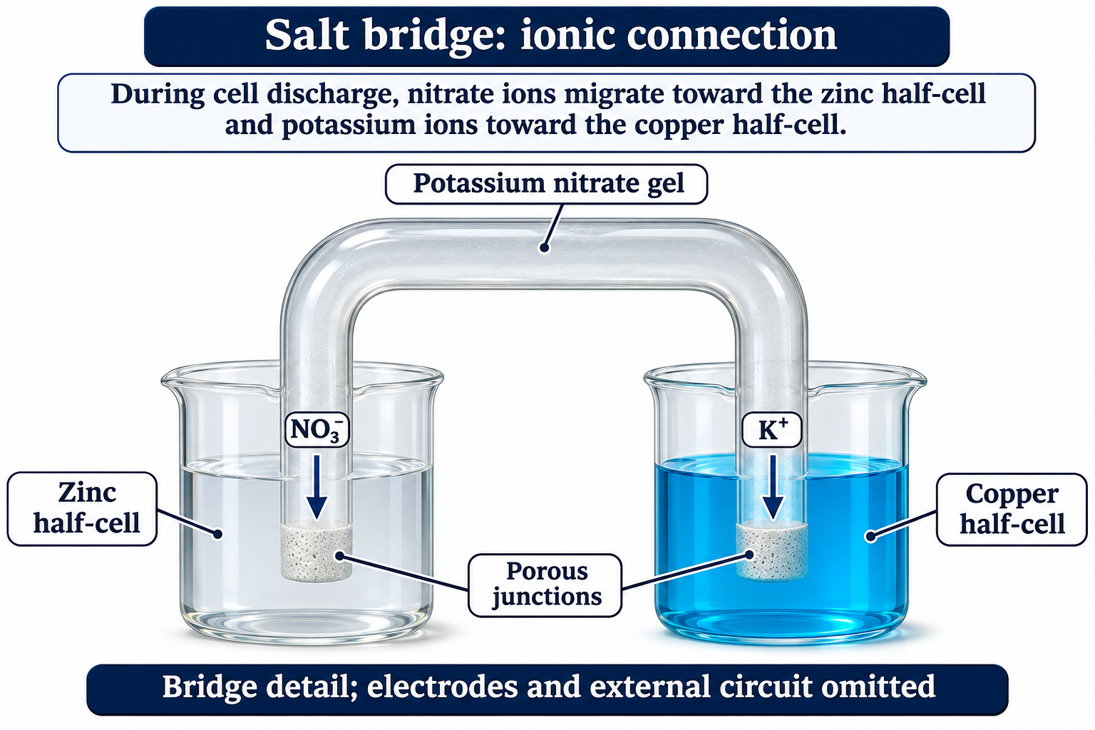
The zinc-and-copper example is illustrative; measured voltage depends on the actual cell conditions.
 CHEMISTRY · C35 · 3 VISUALSElectrolysis with graphite electrodesShow electrode processes during electrolysis of an aqueous solution.
Labelled schematic
Show electrode processes during electrolysis of an aqueous solution.


Realistic apparatus view
Show electrode processes during electrolysis of an aqueous solution.
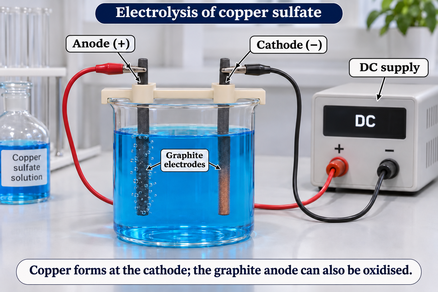

Critical detail
Show electrode processes during electrolysis of an aqueous solution.

Graphite can undergo oxidation, so anode gas should not be assumed to be pure oxygen.
 CHEMISTRY · C36 · 3 VISUALSElectrolysis with gas collectionCollect gases above platinum electrode tips during electrolysis of sodium sulfate solution.
Labelled schematic
Collect gases above platinum electrode tips during electrolysis of sodium sulfate solution.


Realistic apparatus view
Collect gases above platinum electrode tips during electrolysis of sodium sulfate solution.
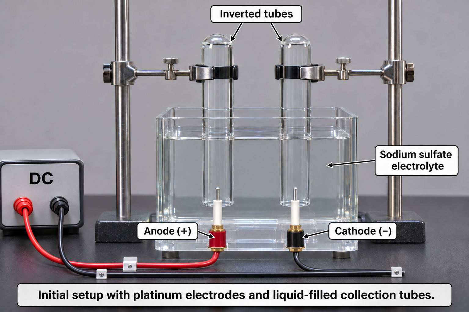

Critical detail
Collect gases above platinum electrode tips during electrolysis of sodium sulfate solution.
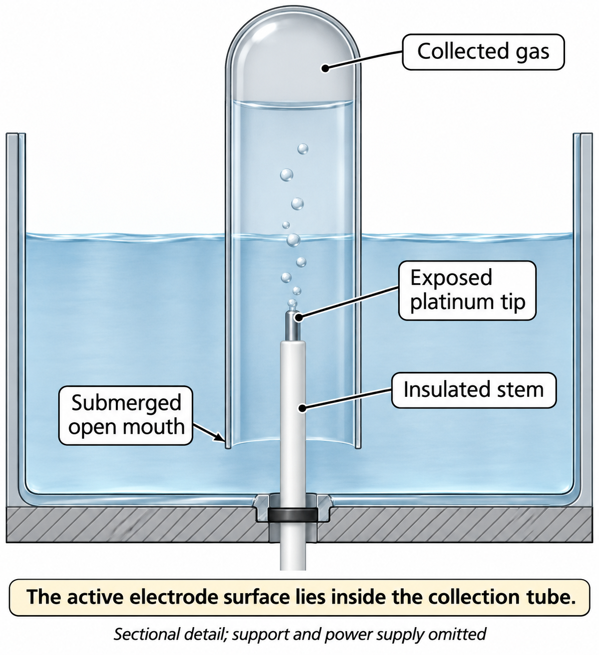
The tubes are shown initially filled; the artwork is not a measured gas-volume ratio.
 CHEMISTRY · C37 · 3 VISUALSElectroplatingDeposit a metal coating on a conducting object using an electrolytic cell.
Labelled schematic
Deposit a metal coating on a conducting object using an electrolytic cell.

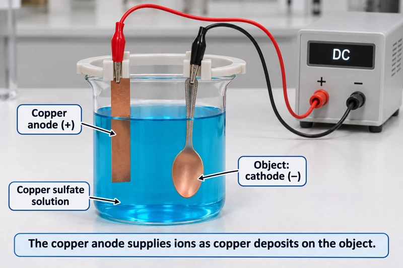
Realistic apparatus view
Deposit a metal coating on a conducting object using an electrolytic cell.

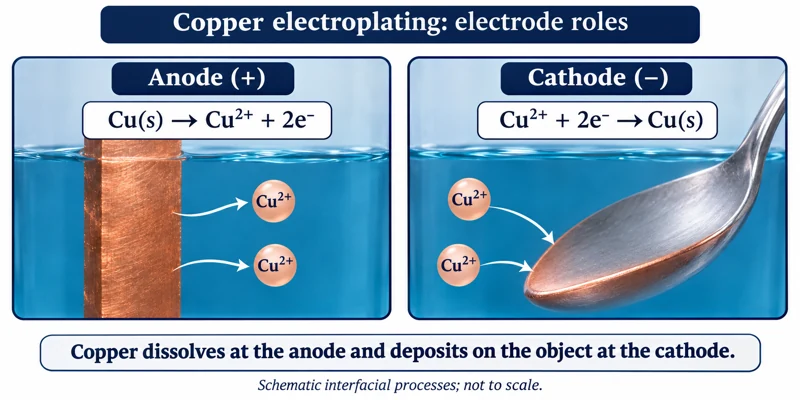
Critical detail
Deposit a metal coating on a conducting object using an electrolytic cell.
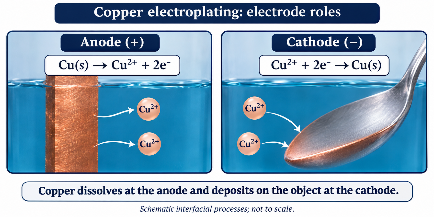
Coating thickness and mass require measurements and are not established by the illustration.
 CHEMISTRY · C38 · 3 VISUALSConductivity testingCompare solution conductivity using a probe and meter.
Labelled schematic
Compare solution conductivity using a probe and meter.
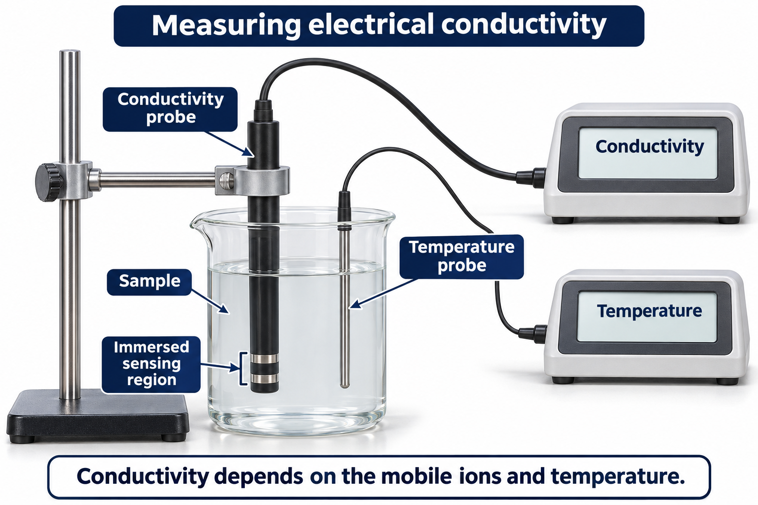

Realistic apparatus view
Compare solution conductivity using a probe and meter.


Critical detail
Compare solution conductivity using a probe and meter.

Conductivity depends on concentration, temperature and cell geometry, not only the identity of dissolved ions.
 CHEMISTRY · C39 · 3 VISUALSFlame-test apparatusIntroduce a small sample into a flame to observe characteristic emission.
Labelled schematic
Introduce a small sample into a flame to observe characteristic emission.
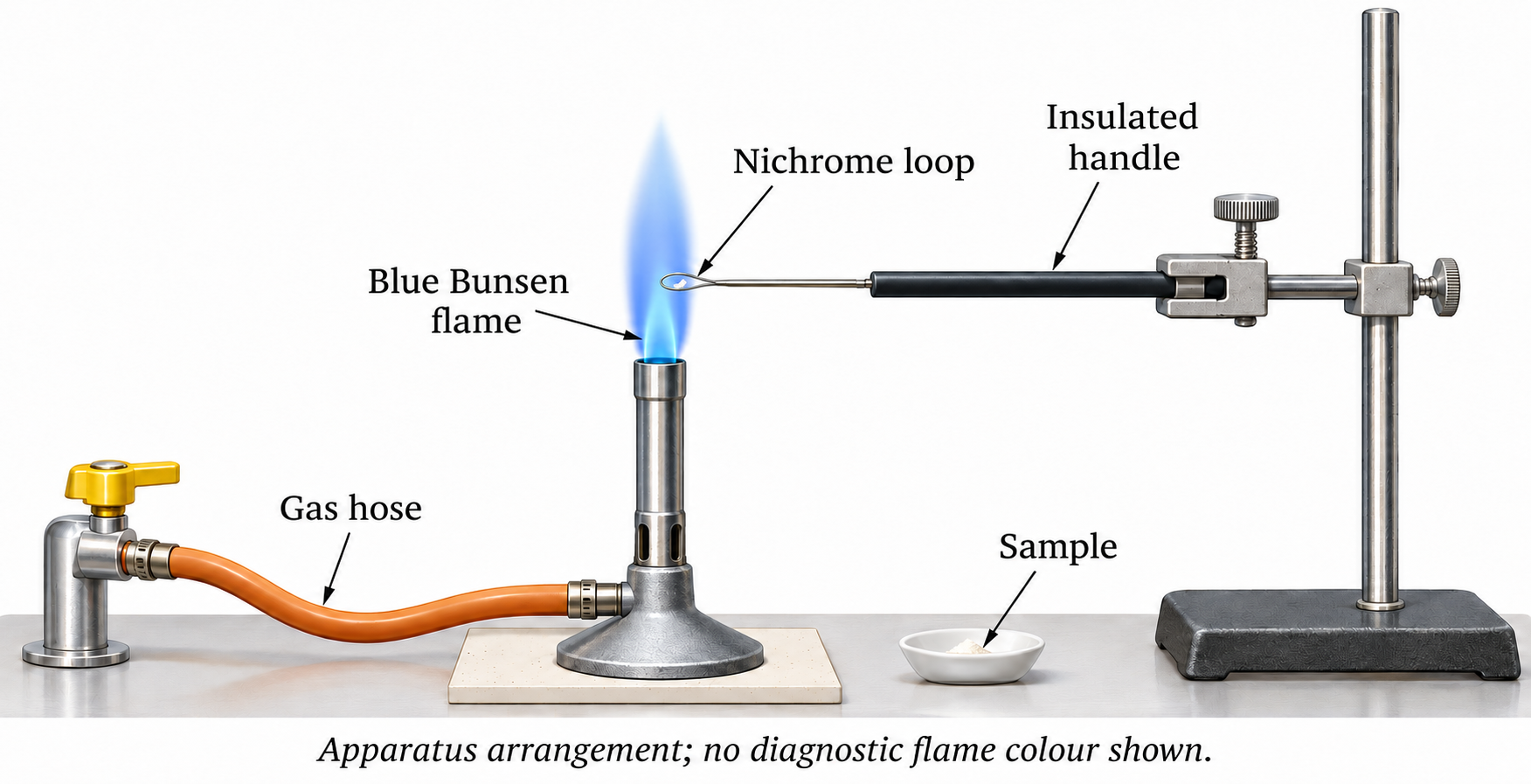

Realistic apparatus view
Introduce a small sample into a flame to observe characteristic emission.


Critical detail
Introduce a small sample into a flame to observe characteristic emission.
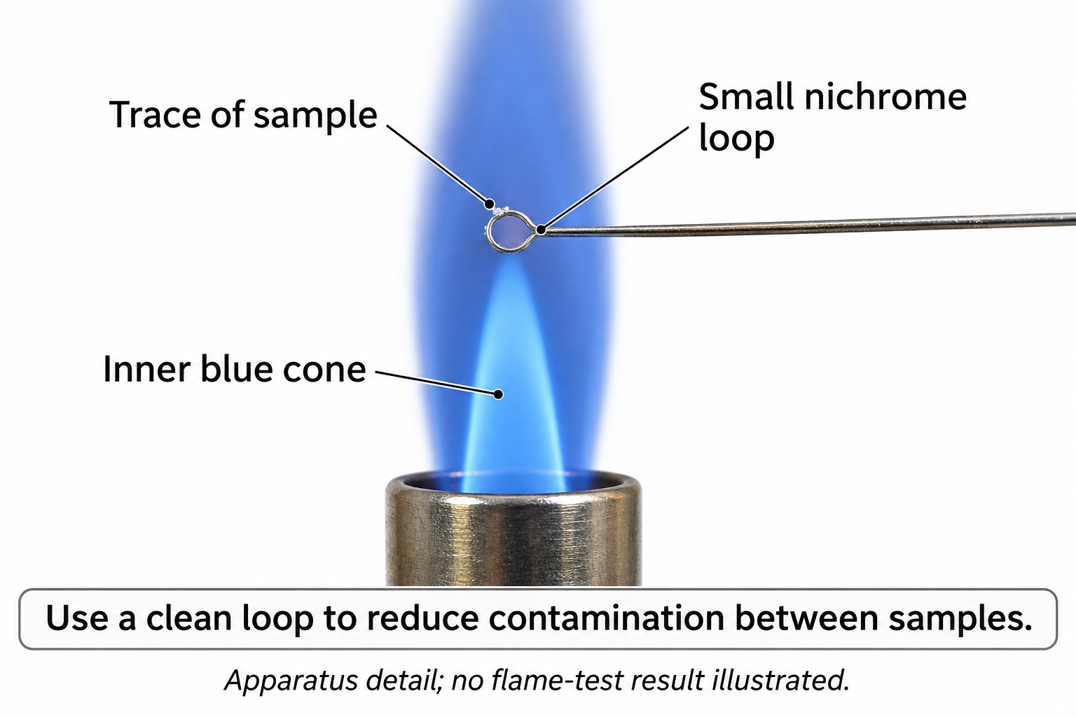
Illustrated colours are not a measured spectrum or sufficient evidence to identify an unknown alone.
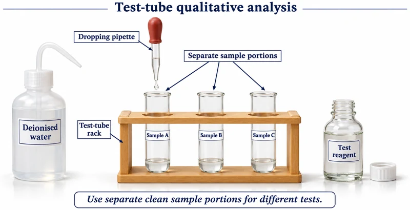 CHEMISTRY · C40 · 3 VISUALSTest-tube qualitative analysisArrange test tubes and dropper reagents for qualitative chemical tests.
Labelled schematic
Arrange test tubes and dropper reagents for qualitative chemical tests.
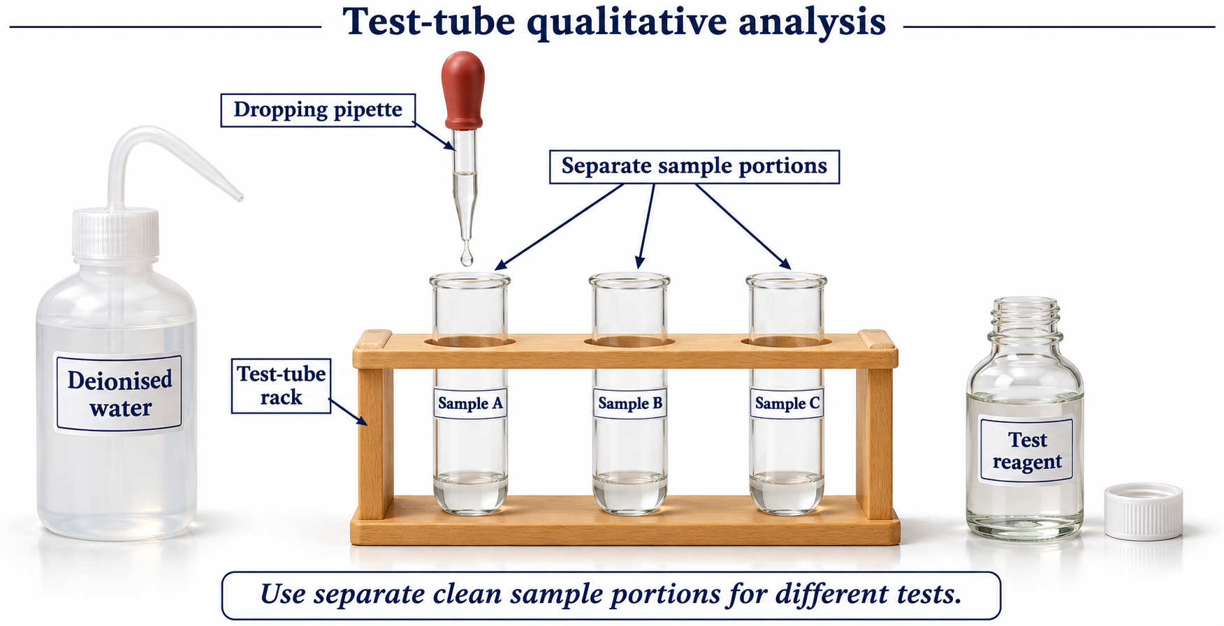

Realistic apparatus view
Arrange test tubes and dropper reagents for qualitative chemical tests.
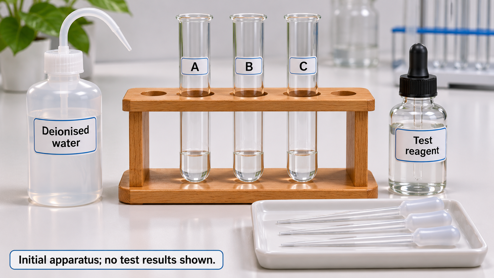

Critical detail
Arrange test tubes and dropper reagents for qualitative chemical tests.

The setup is generic and does not establish a particular unknown or test result.
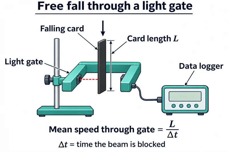 PHYSICS · P01 · 3 VISUALSFree fall through one light gateMeasure the transit time of a falling card through one light gate to estimate its speed.
Labelled schematic
Measure the transit time of a falling card through one light gate to estimate its speed.


Realistic apparatus view
Measure the transit time of a falling card through one light gate to estimate its speed.


Critical detail
Measure the transit time of a falling card through one light gate to estimate its speed.
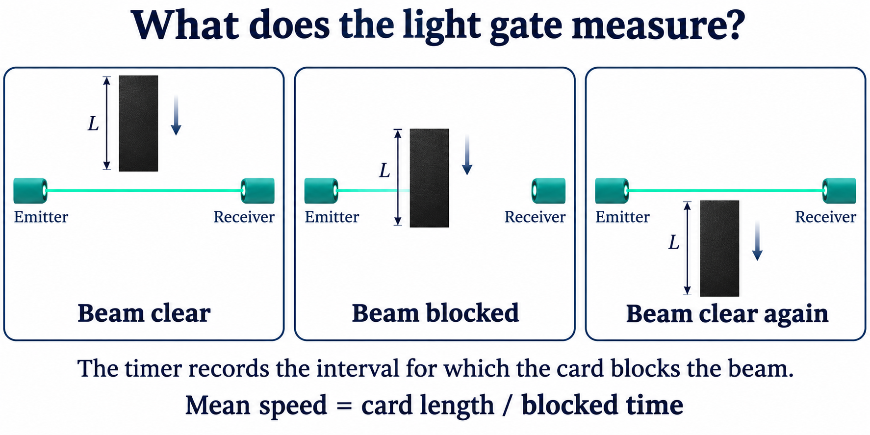
This illustrates transit-speed measurement, not a complete measurement of gravitational acceleration on its own.
 PHYSICS · P02 · 3 VISUALSFree fall through two light gatesCompare motion at two light gates using a falling object and an electronic timing system.
Labelled schematic
Compare motion at two light gates using a falling object and an electronic timing system.


Realistic apparatus view
Compare motion at two light gates using a falling object and an electronic timing system.


Critical detail
Compare motion at two light gates using a falling object and an electronic timing system.

Interpret each timing value according to the gate mode and the object's known dimensions.
 PHYSICS · P04 · 3 VISUALSTrolley motion on a rampUse light gates or motion logging to investigate a trolley's acceleration down a ramp.
Labelled schematic
Use light gates or motion logging to investigate a trolley's acceleration down a ramp.
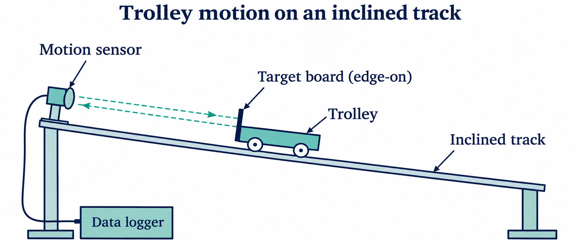

Realistic apparatus view
Use light gates or motion logging to investigate a trolley's acceleration down a ramp.

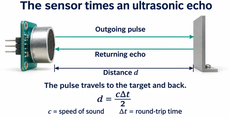
Critical detail
Use light gates or motion logging to investigate a trolley's acceleration down a ramp.

The apparatus represents a measured-motion investigation rather than an ideal frictionless track.
 PHYSICS · P05 · 3 VISUALSNewton's second law trolley systemUse a hanging mass and pulley to accelerate a trolley and investigate force, mass and acceleration.
Labelled schematic
Use a hanging mass and pulley to accelerate a trolley and investigate force, mass and acceleration.


Realistic apparatus view
Use a hanging mass and pulley to accelerate a trolley and investigate force, mass and acceleration.
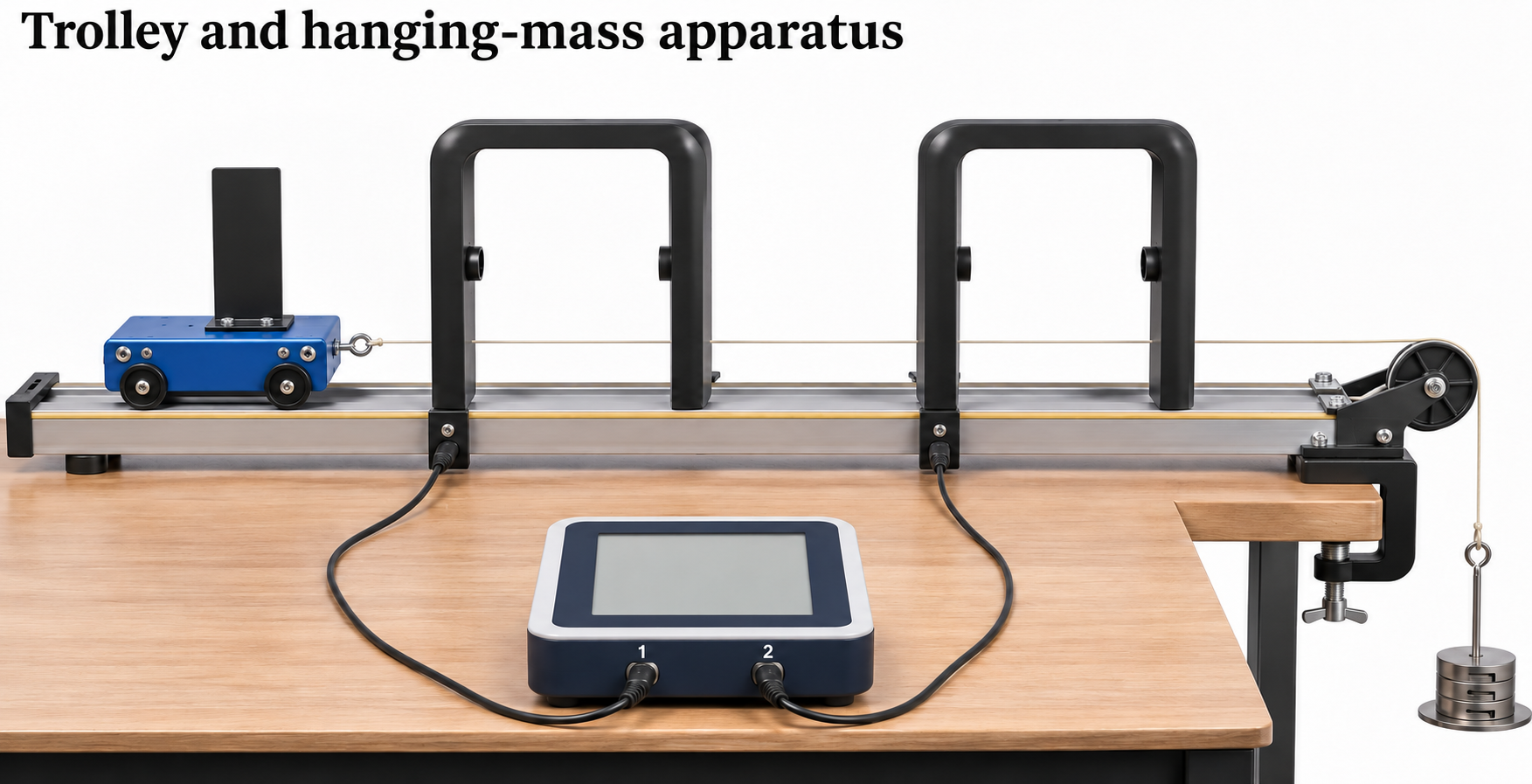

Critical detail
Use a hanging mass and pulley to accelerate a trolley and investigate force, mass and acceleration.

The simple acceleration relation assumes negligible friction and pulley effects and includes the moving hanging mass.
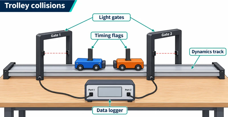 PHYSICS · P06 · 3 VISUALSColliding trolleysMeasure trolley velocities before and after collisions to investigate momentum conservation.
Labelled schematic
Measure trolley velocities before and after collisions to investigate momentum conservation.


Realistic apparatus view
Measure trolley velocities before and after collisions to investigate momentum conservation.

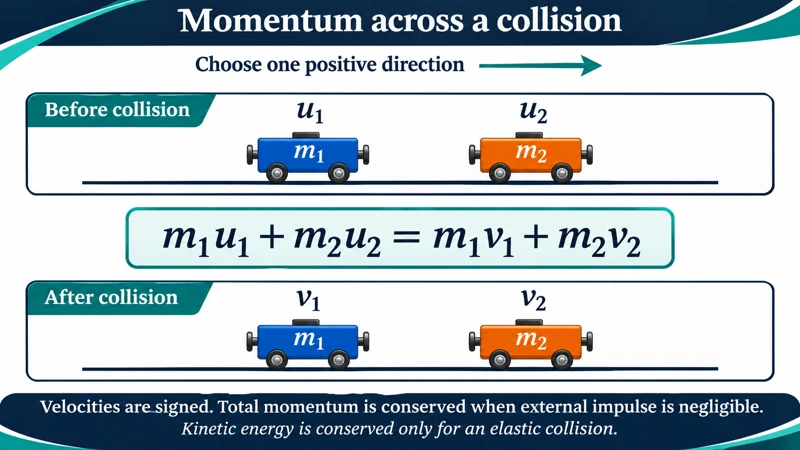
Critical detail
Measure trolley velocities before and after collisions to investigate momentum conservation.
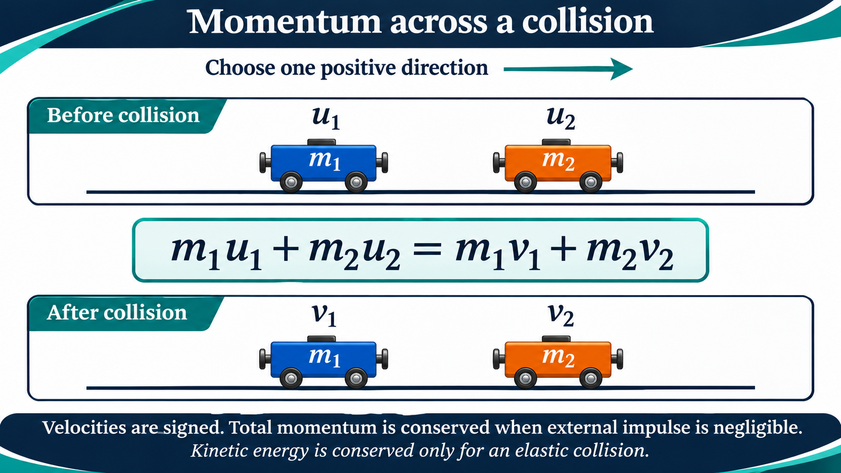
Use signed velocities; approximate conservation requires negligible external impulse during the collision.
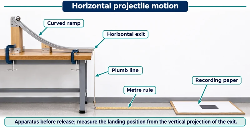 PHYSICS · P07 · 3 VISUALSHorizontal projectile motionUse a ball leaving a horizontal ramp to investigate its landing position and flight.
Labelled schematic
Use a ball leaving a horizontal ramp to investigate its landing position and flight.


Realistic apparatus view
Use a ball leaving a horizontal ramp to investigate its landing position and flight.


Critical detail
Use a ball leaving a horizontal ramp to investigate its landing position and flight.

The trajectory detail uses a point model and vertical displacement of the ball's centre, with air resistance neglected.
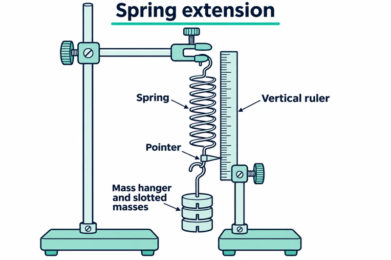 PHYSICS · P08 · 3 VISUALSHooke's lawMeasure spring extension as load is varied.
Labelled schematic
Measure spring extension as load is varied.

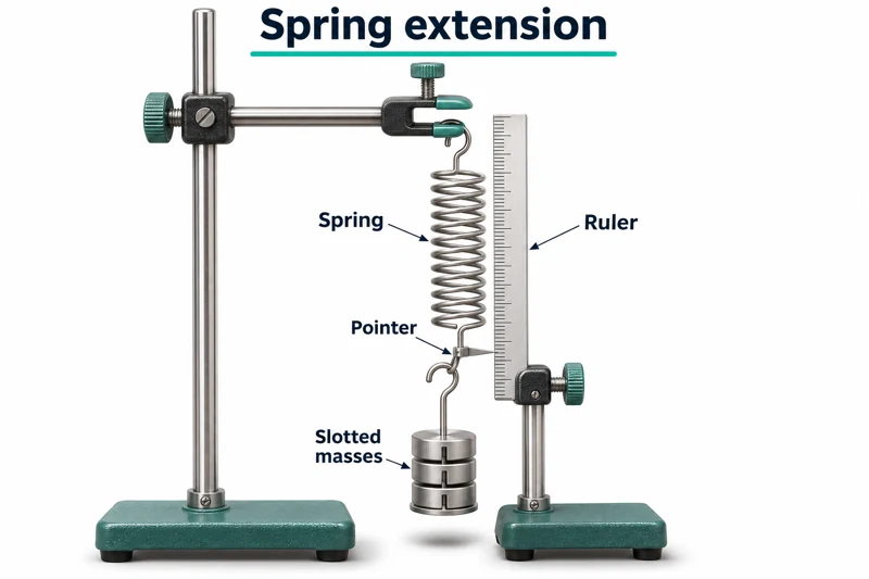
Realistic apparatus view
Measure spring extension as load is varied.


Critical detail
Measure spring extension as load is varied.

A linear force-extension relationship applies only within the spring's proportional range.
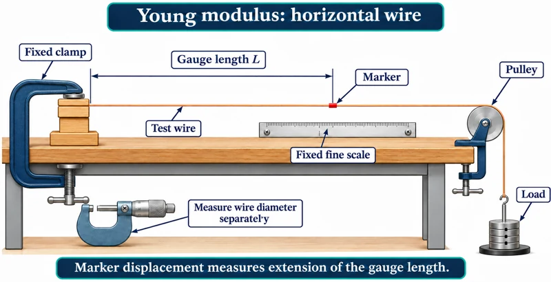 PHYSICS · P09 · 3 VISUALSYoung modulus of a wireMeasure extension of a loaded wire using a marker and fine scale.
Labelled schematic
Measure extension of a loaded wire using a marker and fine scale.


Realistic apparatus view
Measure extension of a loaded wire using a marker and fine scale.


Critical detail
Measure extension of a loaded wire using a marker and fine scale.

The horizontal-wire arrangement measures original length from the fixed clamp to the marker and applies within the elastic linear range.
 PHYSICS · P10 · 3 VISUALSMoments and equilibriumCompare loads and their distances from a pivot when balancing a beam.
Labelled schematic
Compare loads and their distances from a pivot when balancing a beam.


Realistic apparatus view
Compare loads and their distances from a pivot when balancing a beam.

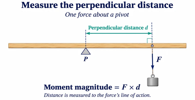
Critical detail
Compare loads and their distances from a pivot when balancing a beam.

Moment arms are perpendicular distances to the forces' lines of action.
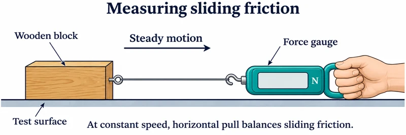 PHYSICS · P11 · 3 VISUALSFriction measurementUse a force gauge to investigate friction between a block and a surface.
Labelled schematic
Use a force gauge to investigate friction between a block and a surface.


Realistic apparatus view
Use a force gauge to investigate friction between a block and a surface.
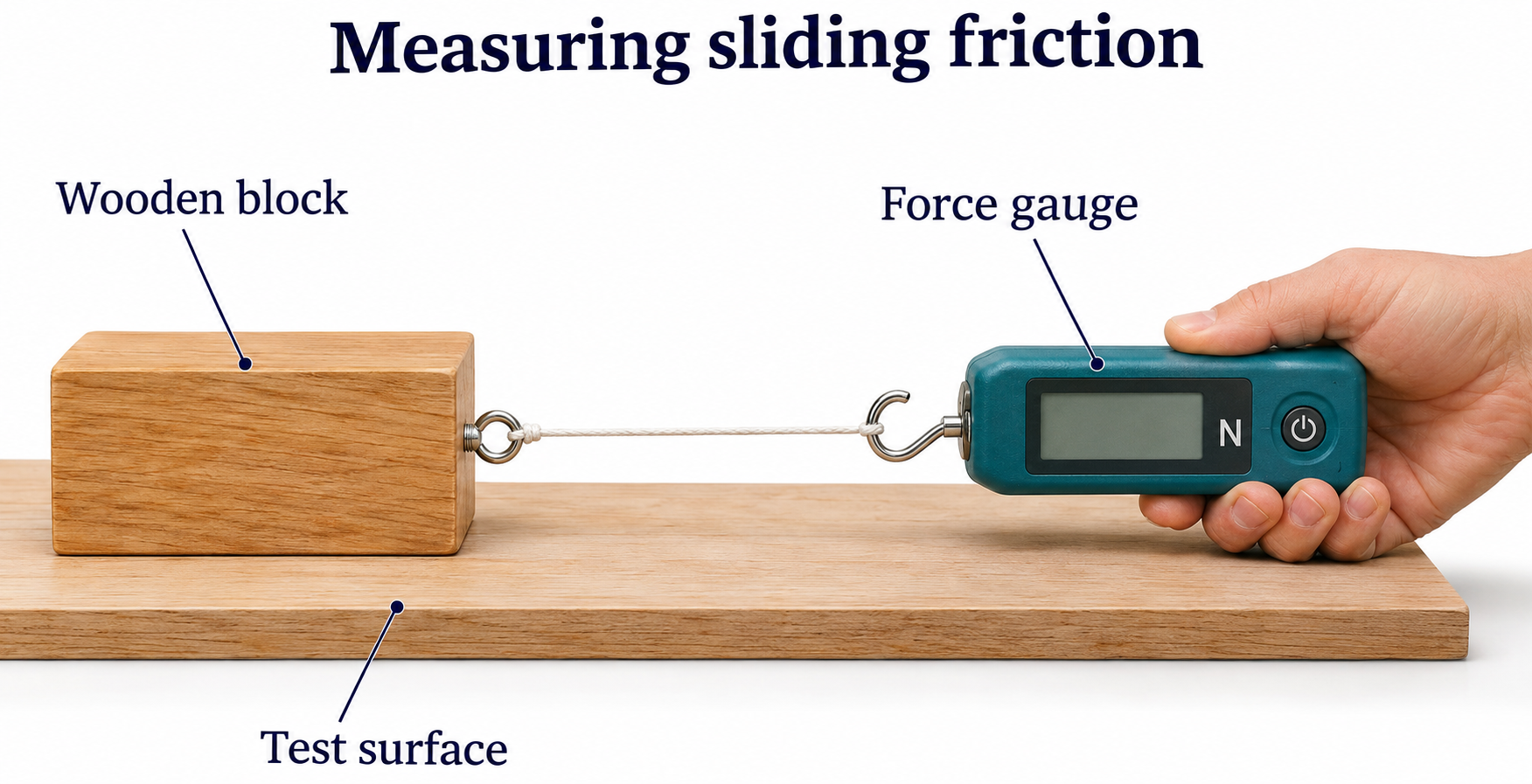

Critical detail
Use a force gauge to investigate friction between a block and a surface.

The horizontal force-balance detail applies to constant speed, not the acceleration of the block.
 PHYSICS · P12 · 3 VISUALSTerminal speed in a liquidTime a falling sphere between marked positions to investigate steady motion in a liquid.
Labelled schematic
Time a falling sphere between marked positions to investigate steady motion in a liquid.
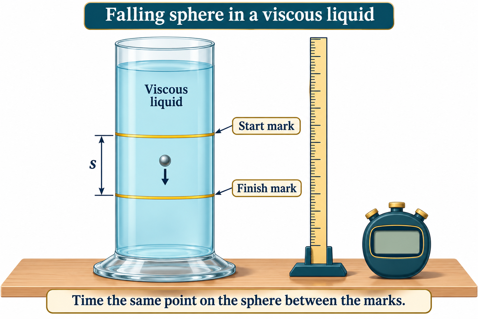

Realistic apparatus view
Time a falling sphere between marked positions to investigate steady motion in a liquid.

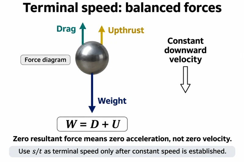
Critical detail
Time a falling sphere between marked positions to investigate steady motion in a liquid.

At terminal speed, weight is balanced by drag and upthrust; steady speed must be established rather than assumed.
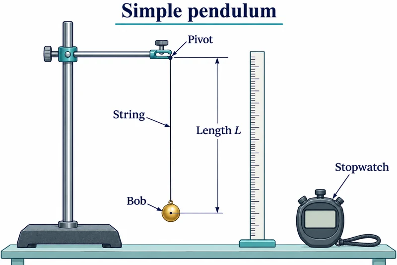 PHYSICS · P13 · 3 VISUALSSimple pendulumMeasure pendulum period while changing its length or other controlled variables.
Labelled schematic
Measure pendulum period while changing its length or other controlled variables.
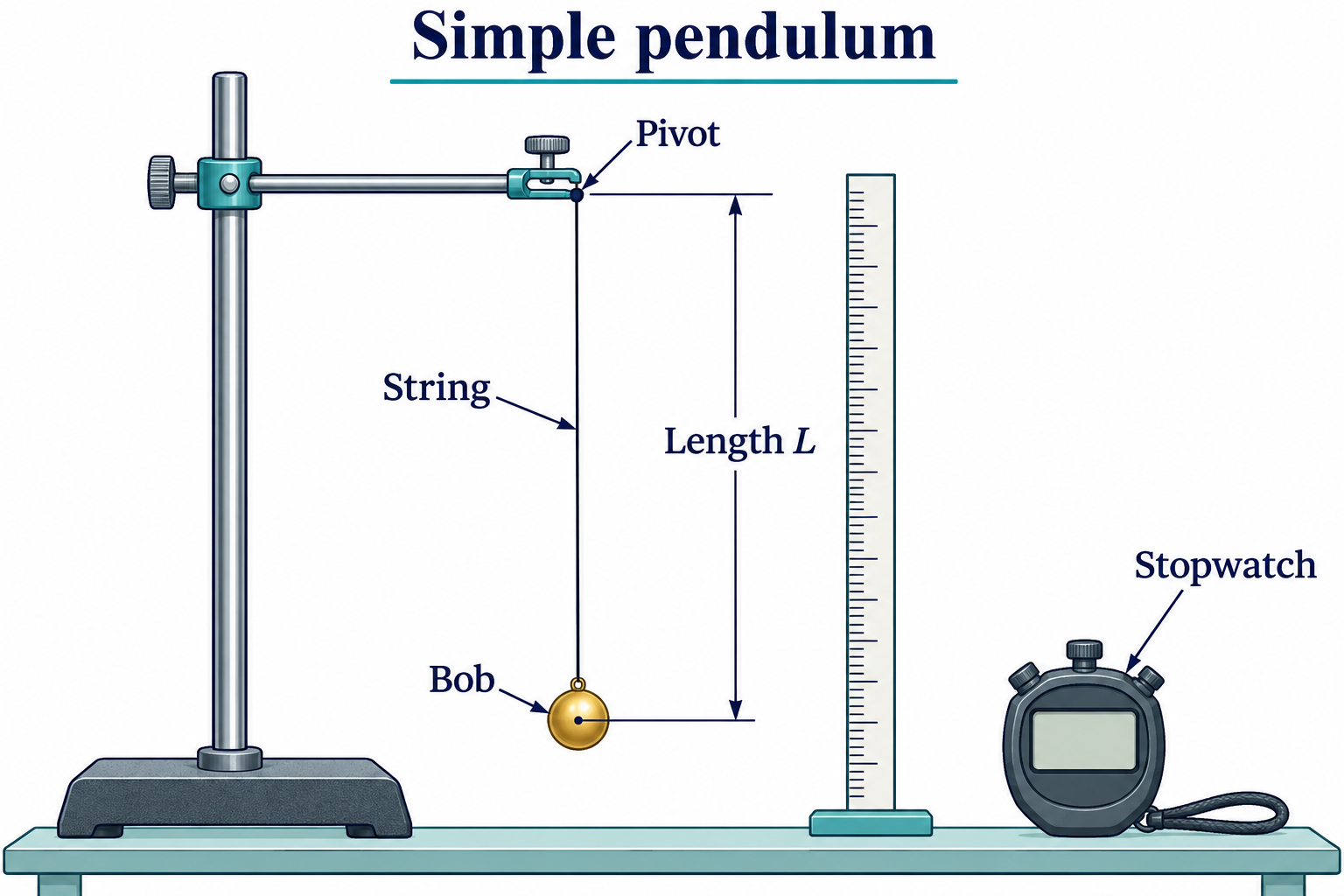

Realistic apparatus view
Measure pendulum period while changing its length or other controlled variables.

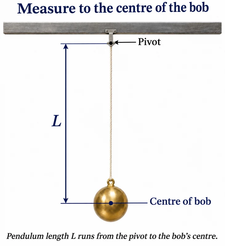
Critical detail
Measure pendulum period while changing its length or other controlled variables.
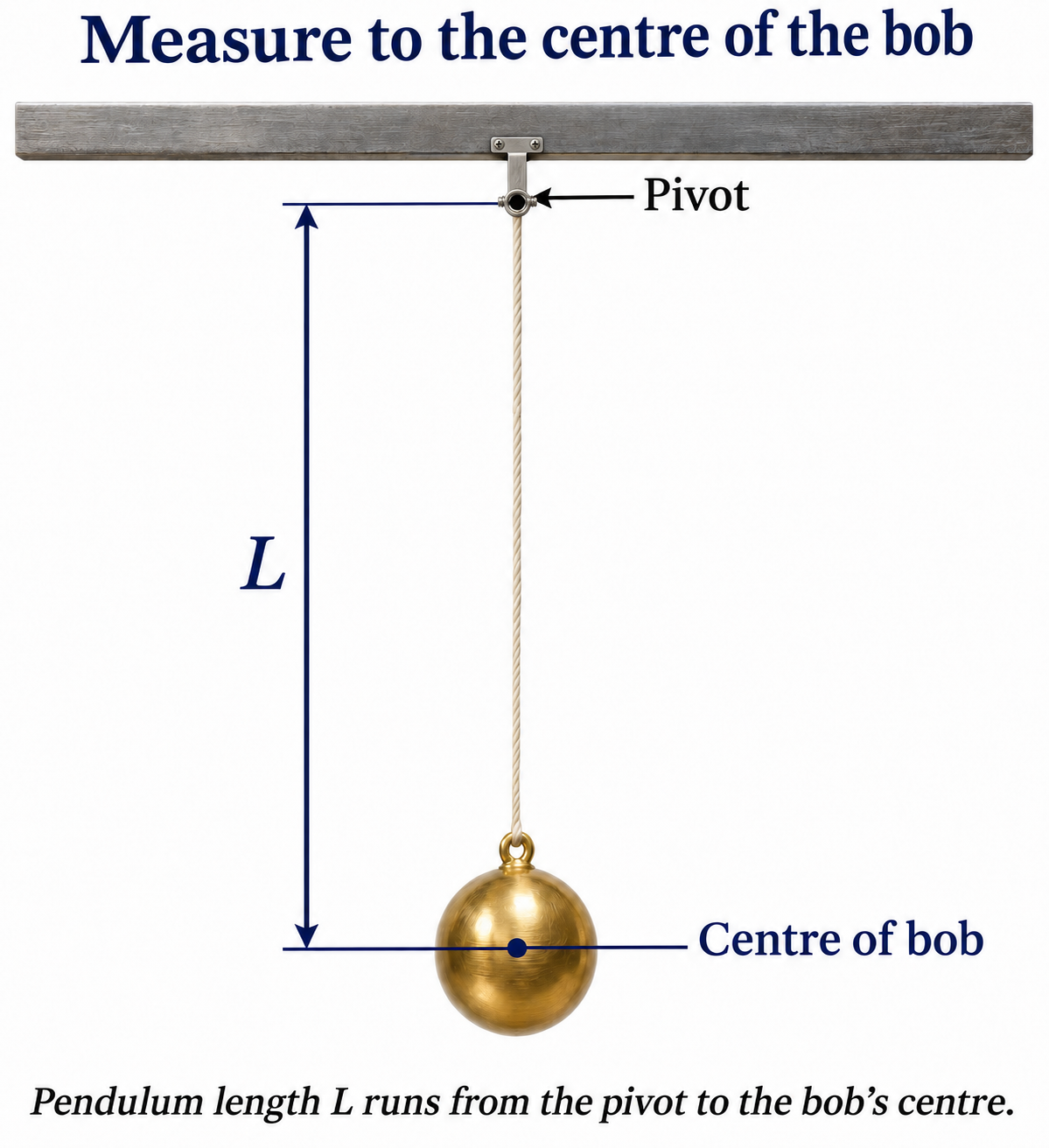
The usual simple-pendulum relation assumes small oscillations and uses pivot-to-bob-centre length.
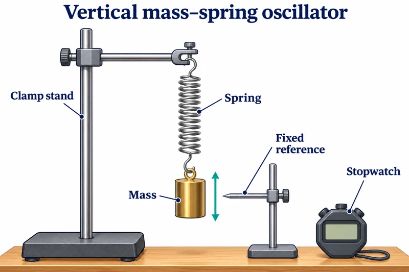 PHYSICS · P14 · 3 VISUALSMass-spring oscillatorMeasure oscillations of a suspended mass on a spring.
Labelled schematic
Measure oscillations of a suspended mass on a spring.


Realistic apparatus view
Measure oscillations of a suspended mass on a spring.


Critical detail
Measure oscillations of a suspended mass on a spring.

The ideal model assumes small linear oscillations; spring mass and damping can affect measured periods.
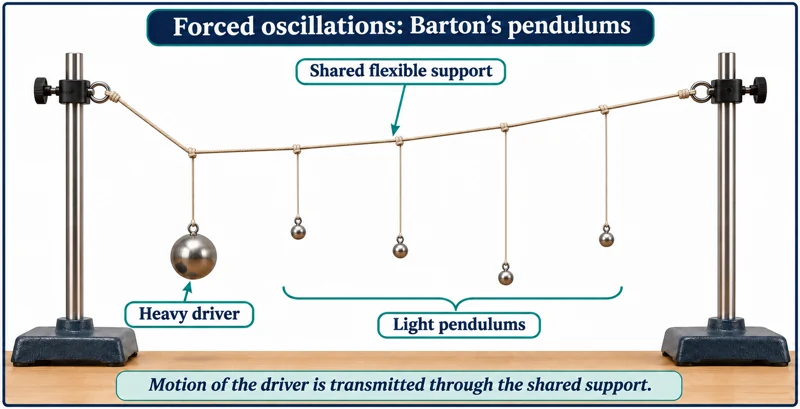 PHYSICS · P15 · 3 VISUALSBarton pendulums and resonanceUse a driving pendulum and suspended pendulums to demonstrate coupled oscillations and resonance.
Labelled schematic
Use a driving pendulum and suspended pendulums to demonstrate coupled oscillations and resonance.


Realistic apparatus view
Use a driving pendulum and suspended pendulums to demonstrate coupled oscillations and resonance.
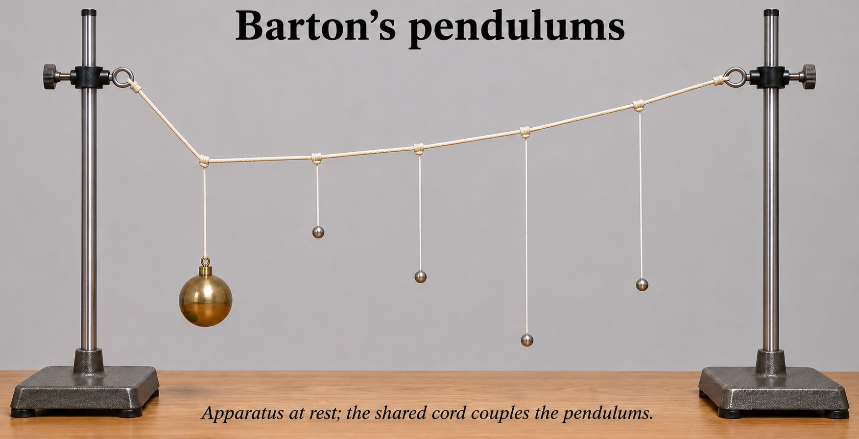

Critical detail
Use a driving pendulum and suspended pendulums to demonstrate coupled oscillations and resonance.
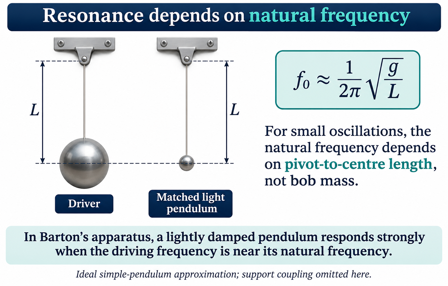
This is the Barton-pendulum variant; damping and coupling affect the response.
 PHYSICS · P16 · 3 VISUALSStanding waves on a stringDrive a tensioned string to investigate resonant modes and wavelength.
Labelled schematic
Drive a tensioned string to investigate resonant modes and wavelength.


Realistic apparatus view
Drive a tensioned string to investigate resonant modes and wavelength.


Critical detail
Drive a tensioned string to investigate resonant modes and wavelength.

Adjacent nodes are half a wavelength apart; the illustrated snapshots are not a recorded motion trace.
 PHYSICS · P17 · 3 VISUALSRipple tankGenerate water waves and use a projected pattern to examine wavelength and propagation.
Labelled schematic
Generate water waves and use a projected pattern to examine wavelength and propagation.
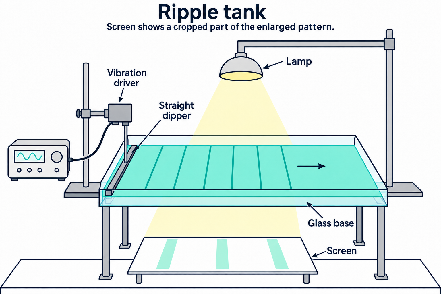

Realistic apparatus view
Generate water waves and use a projected pattern to examine wavelength and propagation.

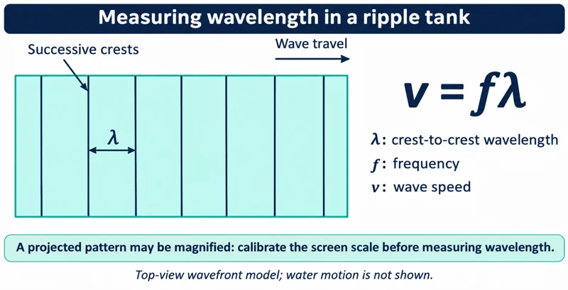
Critical detail
Generate water waves and use a projected pattern to examine wavelength and propagation.

Projected distances require calibration before they represent distances in the tank.
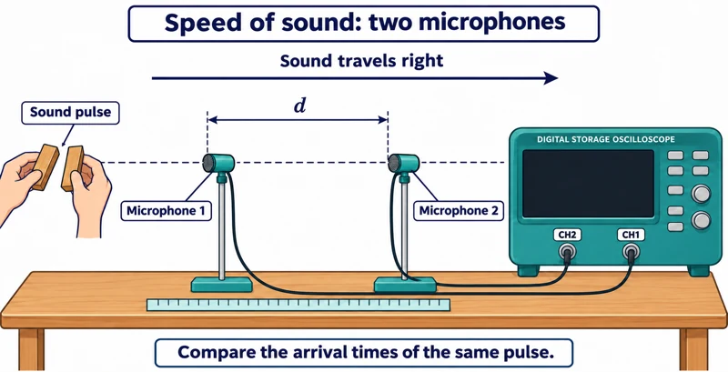 PHYSICS · P18 · 3 VISUALSSpeed of sound with two microphonesMeasure the delay between sound pulses reaching two spaced microphones.
Labelled schematic
Measure the delay between sound pulses reaching two spaced microphones.


Realistic apparatus view
Measure the delay between sound pulses reaching two spaced microphones.


Critical detail
Measure the delay between sound pulses reaching two spaced microphones.

Distance is measured between the sensing positions; use the corresponding time delay rather than a waveform period.
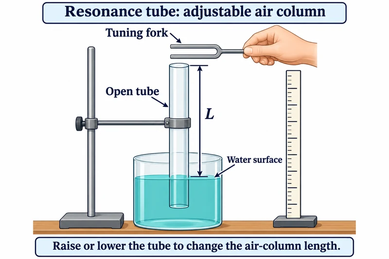 PHYSICS · P19 · 3 VISUALSResonance tubeAdjust an air-column length to locate sound resonances.
Labelled schematic
Adjust an air-column length to locate sound resonances.


Realistic apparatus view
Adjust an air-column length to locate sound resonances.

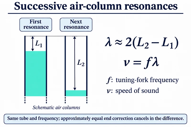
Critical detail
Adjust an air-column length to locate sound resonances.
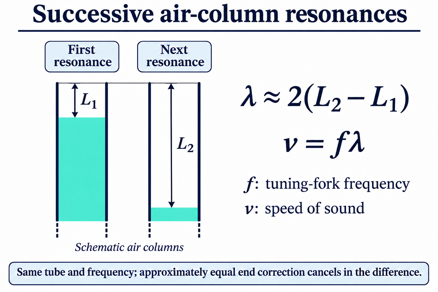
End correction affects resonance lengths, and the illustrated bath does not guarantee two resonances for an unspecified tuning fork.
 PHYSICS · P20 · 3 VISUALSSound signals on an oscilloscopeDisplay a microphone's electrical signal to compare sound frequency and amplitude.
Labelled schematic
Display a microphone's electrical signal to compare sound frequency and amplitude.


Realistic apparatus view
Display a microphone's electrical signal to compare sound frequency and amplitude.


Critical detail
Display a microphone's electrical signal to compare sound frequency and amplitude.

The trace represents the microphone signal, not a picture of air-particle motion or a standing-wave pattern.
 PHYSICS · P21 · 3 VISUALSRefraction through a transparent blockTrace light through a parallel-sided block and compare angles at its boundaries.
Labelled schematic
Trace light through a parallel-sided block and compare angles at its boundaries.


Realistic apparatus view
Trace light through a parallel-sided block and compare angles at its boundaries.
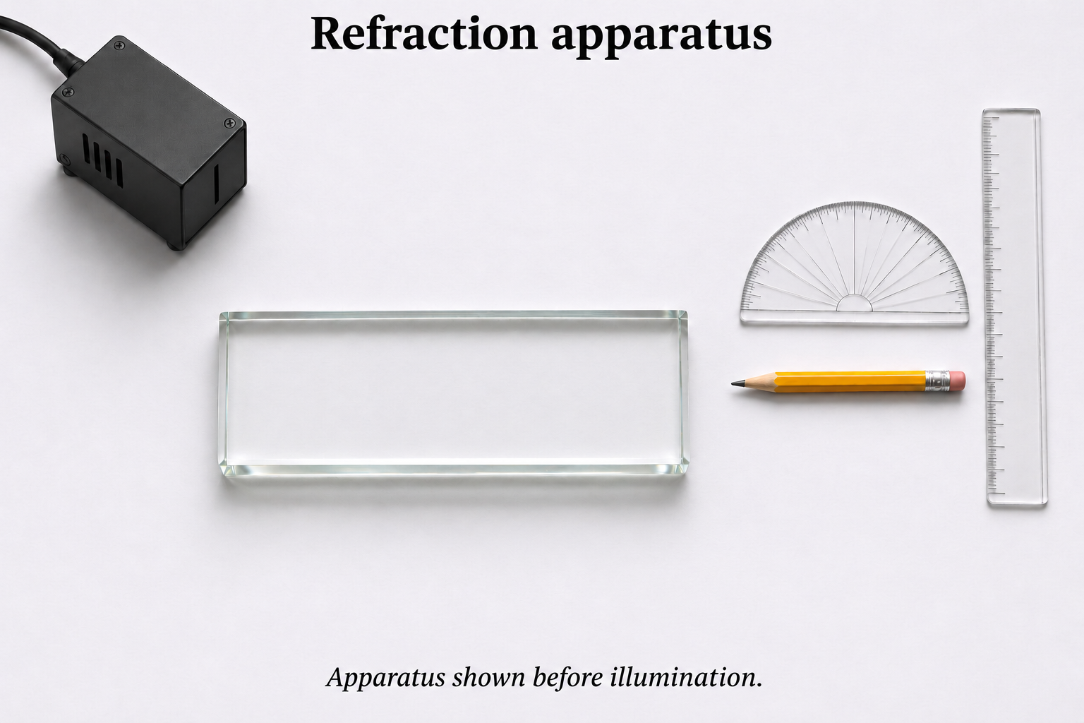
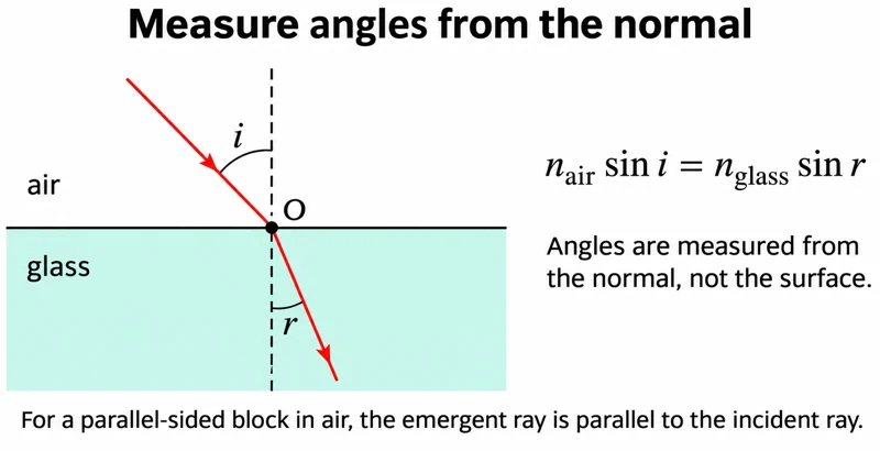
Critical detail
Trace light through a parallel-sided block and compare angles at its boundaries.

Angles are measured from the normal; the realistic view shows apparatus before illumination rather than measured rays.
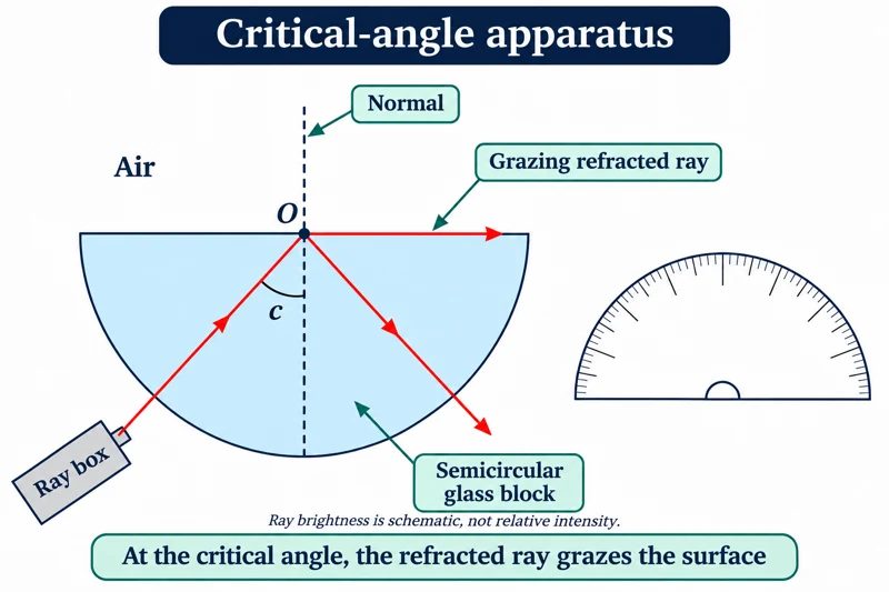 PHYSICS · P22 · 3 VISUALSCritical angle with a semicircular blockDirect light through a semicircular block to investigate the onset of total internal reflection.
Labelled schematic
Direct light through a semicircular block to investigate the onset of total internal reflection.


Realistic apparatus view
Direct light through a semicircular block to investigate the onset of total internal reflection.
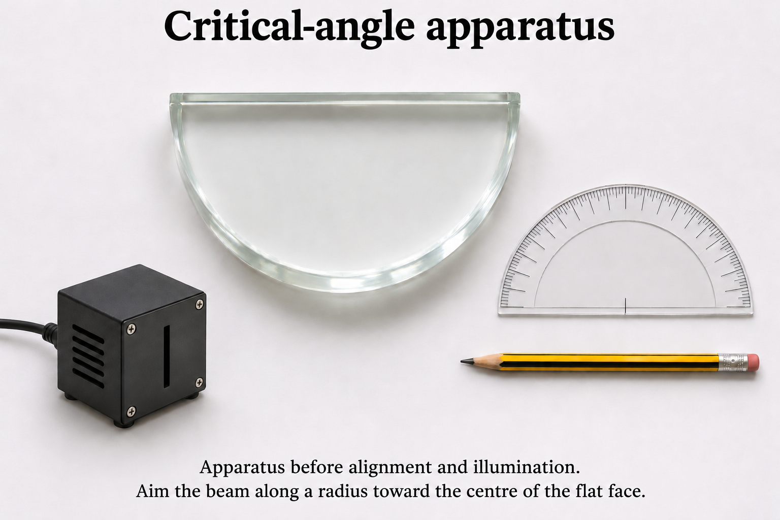

Critical detail
Direct light through a semicircular block to investigate the onset of total internal reflection.

The critical angle is measured inside the higher-index medium from the normal; the realistic view is before final alignment.
 PHYSICS · P23 · 3 VISUALSLens and screen on an optical benchForm a real image on a screen and compare object and image distances.
Labelled schematic
Form a real image on a screen and compare object and image distances.


Realistic apparatus view
Form a real image on a screen and compare object and image distances.


Critical detail
Form a real image on a screen and compare object and image distances.

The ray model uses a thin lens; the image position must coincide with the screen for a focused projection.
 PHYSICS · P24 · 3 VISUALSDouble-slit interferenceIlluminate two slits coherently and examine the fringe pattern on a screen.
Labelled schematic
Illuminate two slits coherently and examine the fringe pattern on a screen.
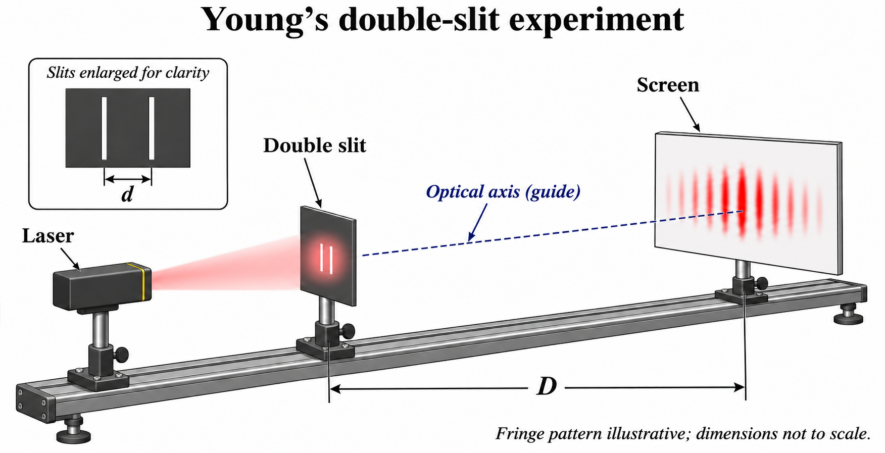

Realistic apparatus view
Illuminate two slits coherently and examine the fringe pattern on a screen.

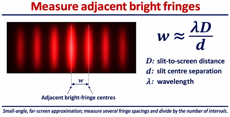
Critical detail
Illuminate two slits coherently and examine the fringe pattern on a screen.

The usual fringe-spacing relation uses the small-angle approximation; the realistic view is before illumination.
 PHYSICS · P25 · 3 VISUALSDiffraction gratingUse a diffraction grating to relate diffraction angle to wavelength.
Labelled schematic
Use a diffraction grating to relate diffraction angle to wavelength.
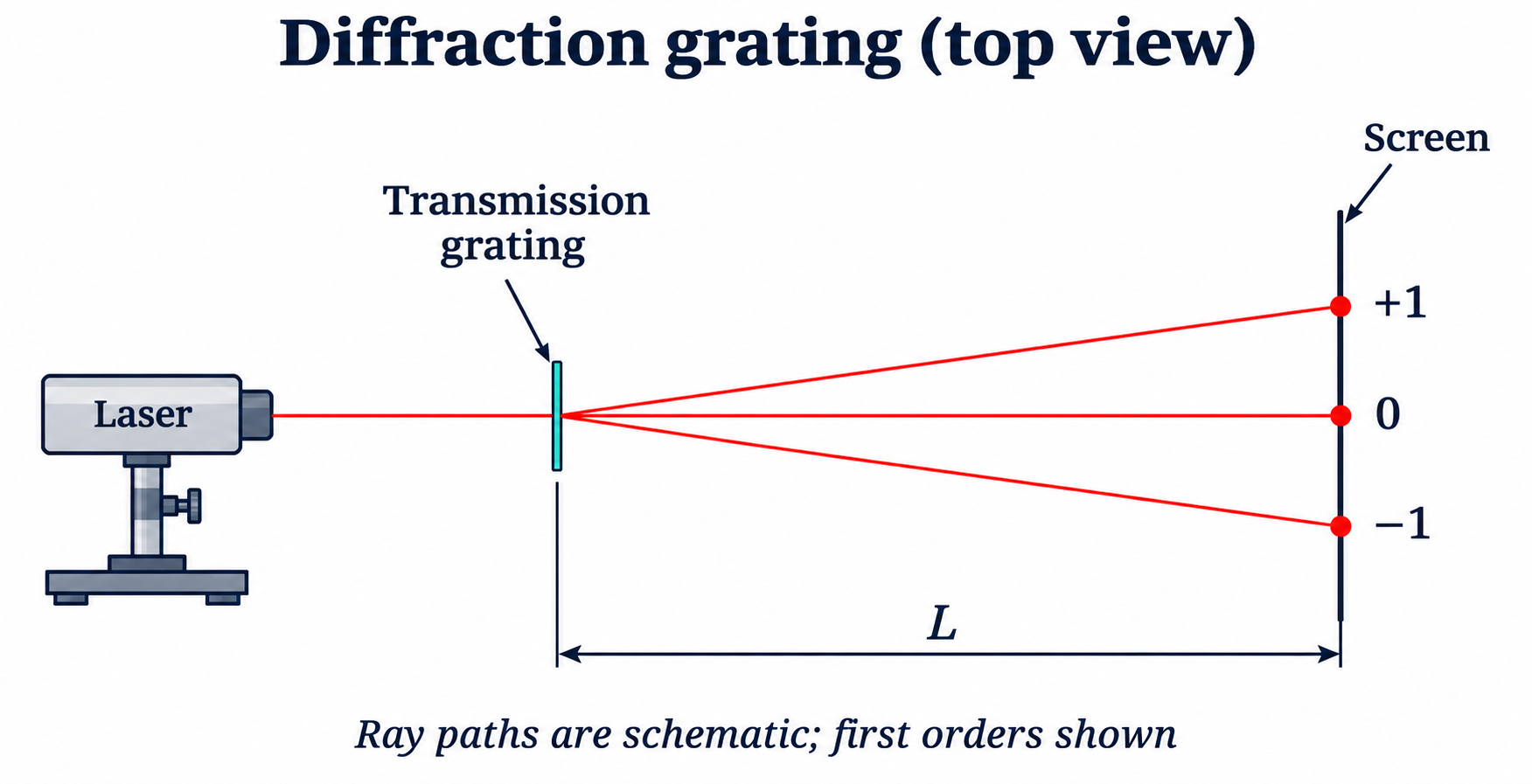

Realistic apparatus view
Use a diffraction grating to relate diffraction angle to wavelength.
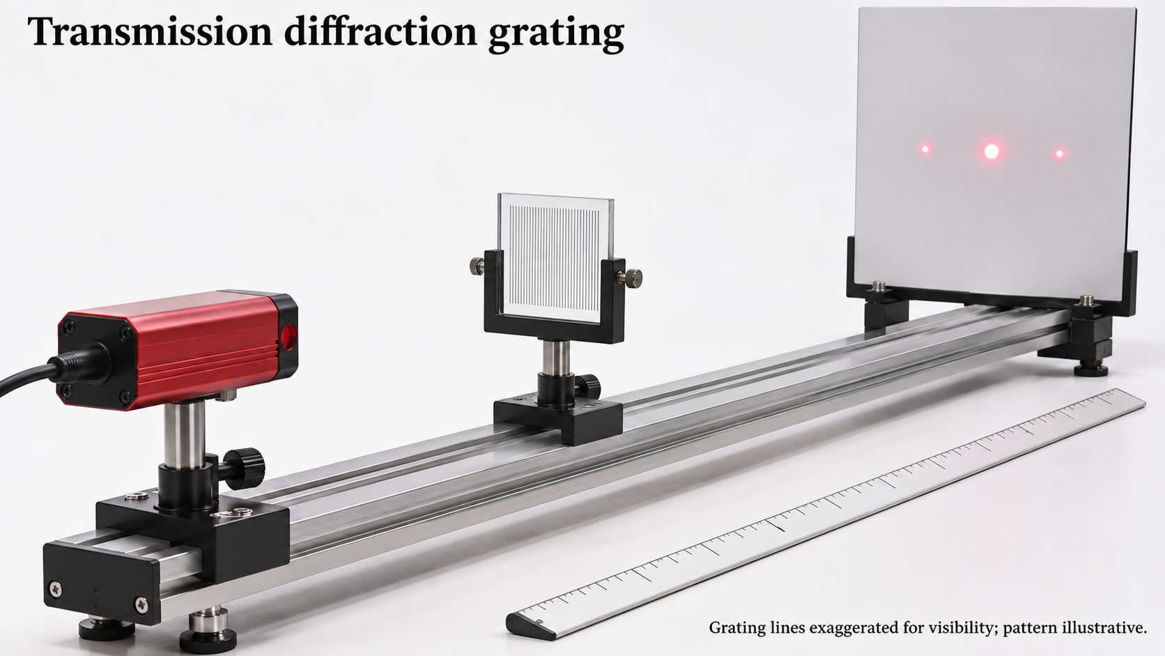
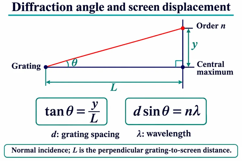
Critical detail
Use a diffraction grating to relate diffraction angle to wavelength.

The illustrated relation assumes normal incidence; screen displacement must be converted to an angle using the actual geometry.
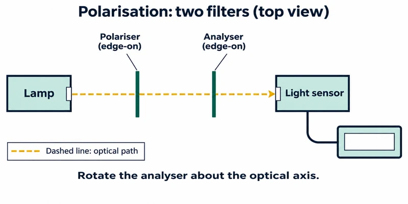 PHYSICS · P26 · 3 VISUALSPolarisation with two filtersCompare transmitted light as the angle between two polarisers changes.
Labelled schematic
Compare transmitted light as the angle between two polarisers changes.
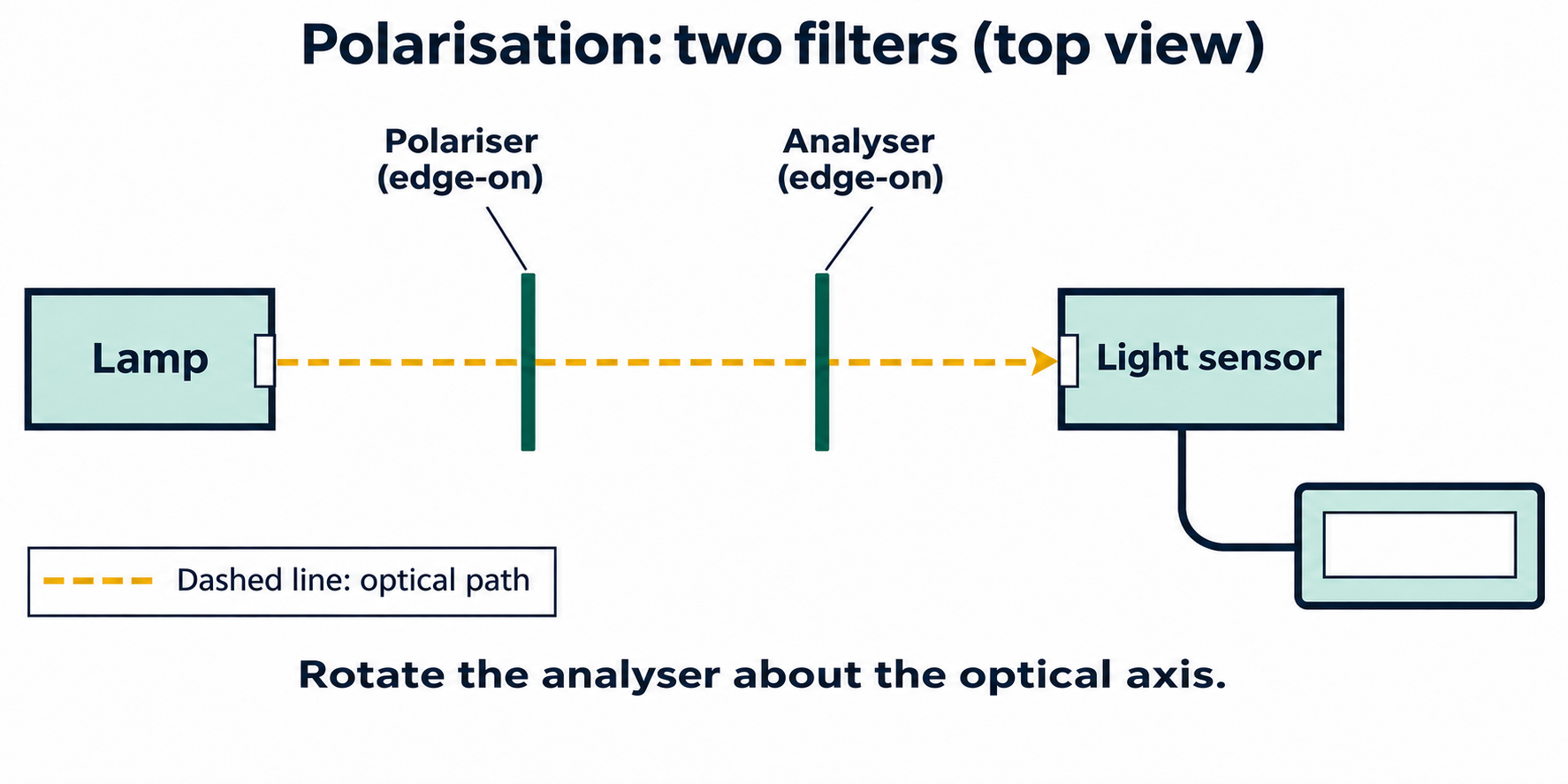

Realistic apparatus view
Compare transmitted light as the angle between two polarisers changes.
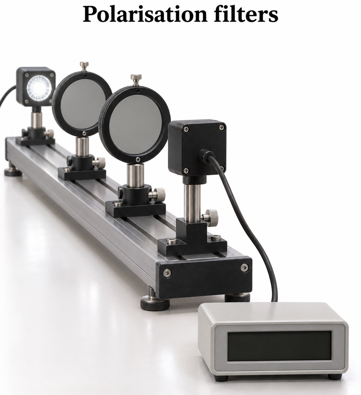
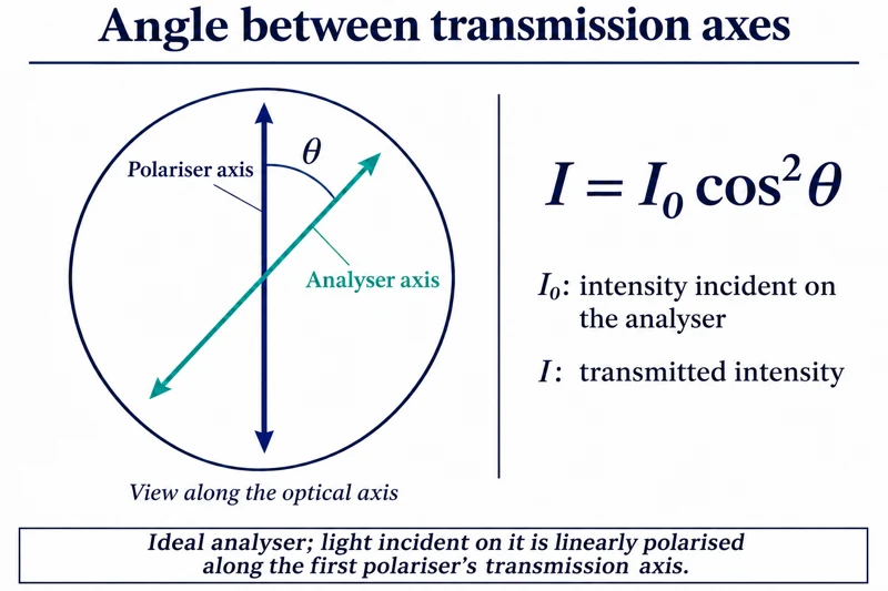
Critical detail
Compare transmitted light as the angle between two polarisers changes.

Ideal polariser relationships do not account for all losses in real filters.
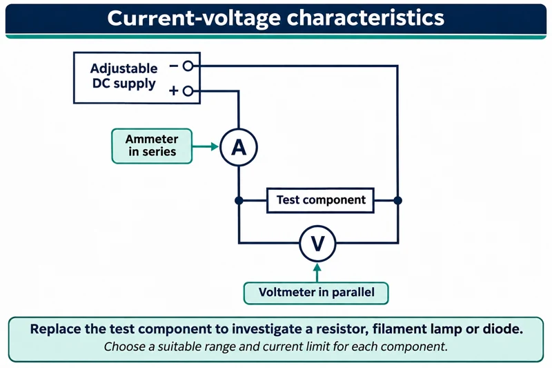 PHYSICS · P27 · 3 VISUALSCurrent-voltage characteristicsMeasure current and potential difference for a test component in a controlled circuit.
Labelled schematic
Measure current and potential difference for a test component in a controlled circuit.


Realistic apparatus view
Measure current and potential difference for a test component in a controlled circuit.
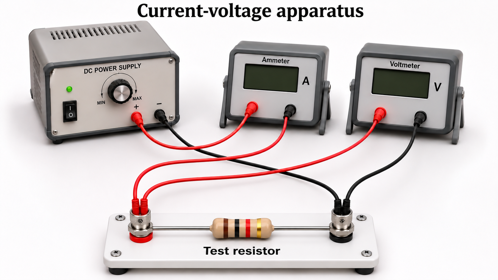

Critical detail
Measure current and potential difference for a test component in a controlled circuit.

The resistor example's linear relation assumes constant temperature; not every component is ohmic.
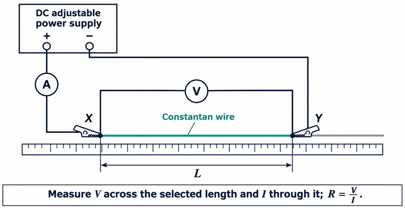 PHYSICS · P28 · 3 VISUALSResistance of a wireMeasure current and potential difference across a selected wire length.
Labelled schematic
Measure current and potential difference across a selected wire length.


Realistic apparatus view
Measure current and potential difference across a selected wire length.
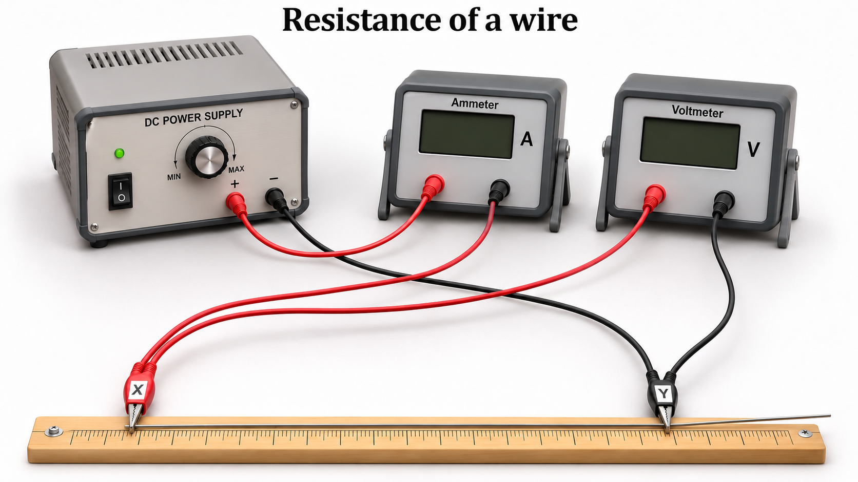

Critical detail
Measure current and potential difference across a selected wire length.

Resistivity calculations require wire cross-sectional area and controlled temperature; contact resistance can affect results.
 PHYSICS · P29 · 3 VISUALSSeries and parallel circuitsCompare how components are connected in series and parallel arrangements.
Labelled schematic
Compare how components are connected in series and parallel arrangements.


Realistic apparatus view
Compare how components are connected in series and parallel arrangements.
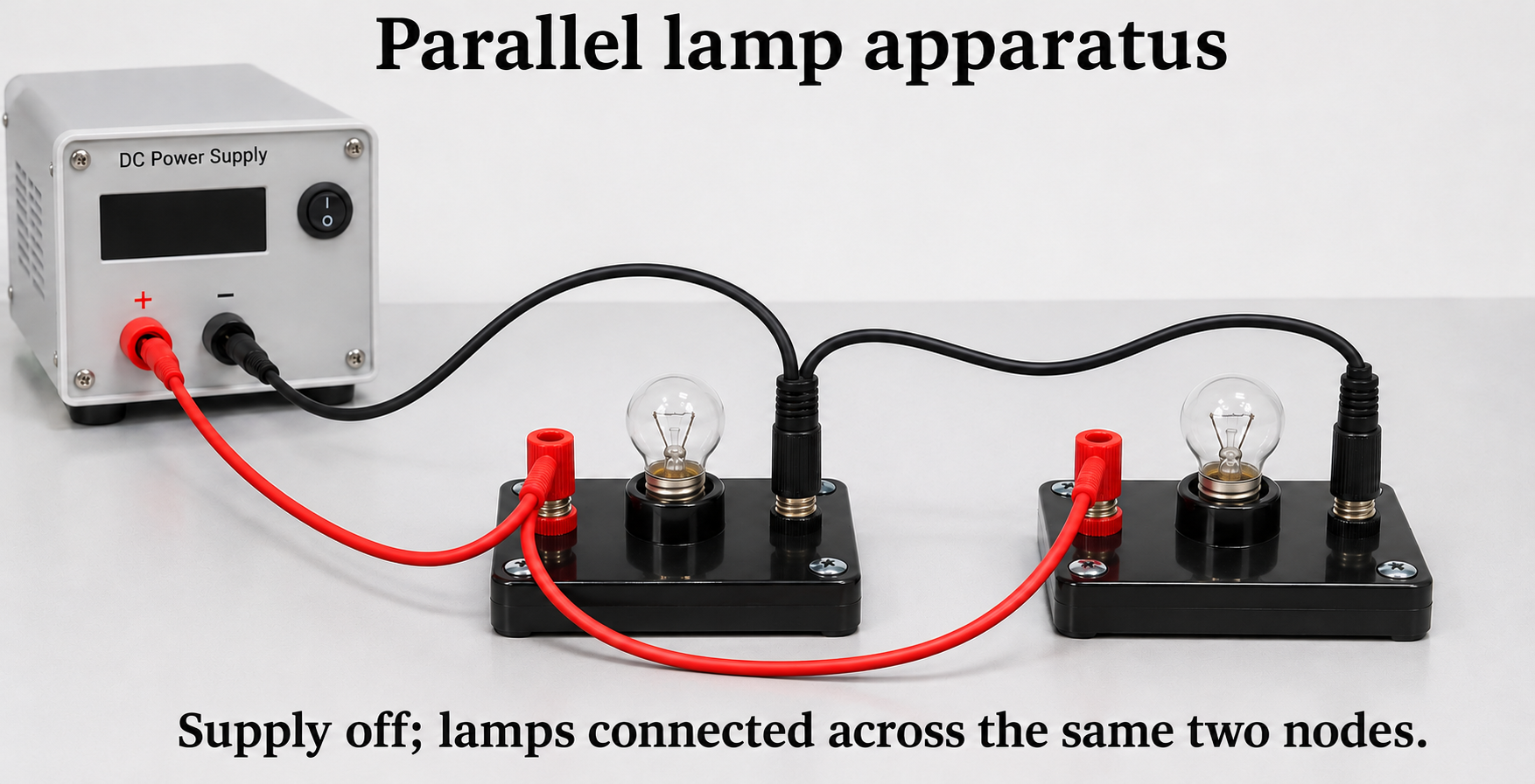

Critical detail
Compare how components are connected in series and parallel arrangements.

Schematic and physical layouts represent connectivity rather than measured component values.
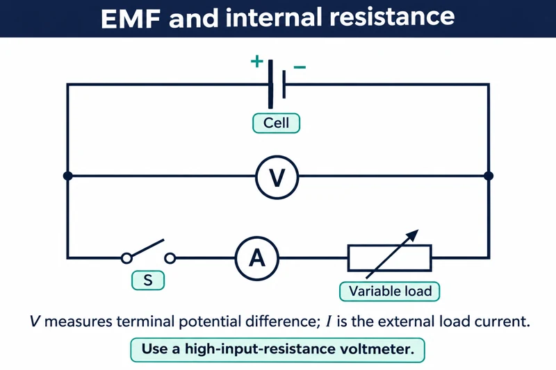 PHYSICS · P30 · 3 VISUALSEMF and internal resistanceVary a cell's load and measure terminal potential difference and current.
Labelled schematic
Vary a cell's load and measure terminal potential difference and current.


Realistic apparatus view
Vary a cell's load and measure terminal potential difference and current.
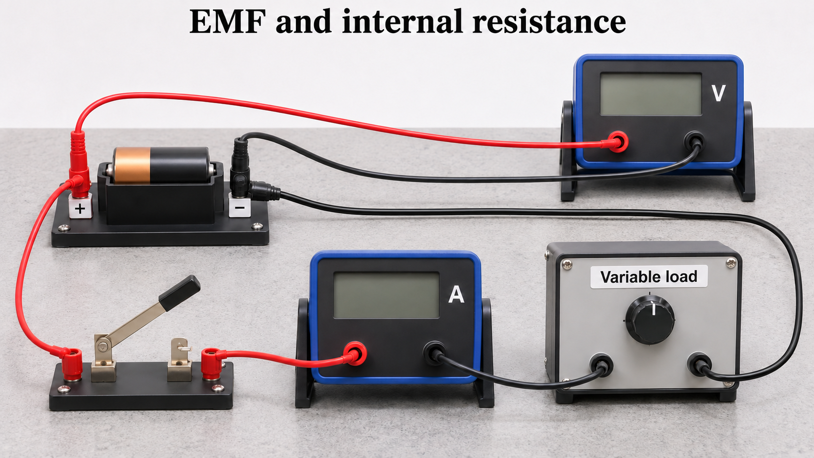

Critical detail
Vary a cell's load and measure terminal potential difference and current.

The straight-line model treats EMF and internal resistance as approximately constant over the measurements.
 PHYSICS · P31 · 3 VISUALSPotential dividerUse two resistors to obtain an output voltage from a supply.
Labelled schematic
Use two resistors to obtain an output voltage from a supply.


Realistic apparatus view
Use two resistors to obtain an output voltage from a supply.
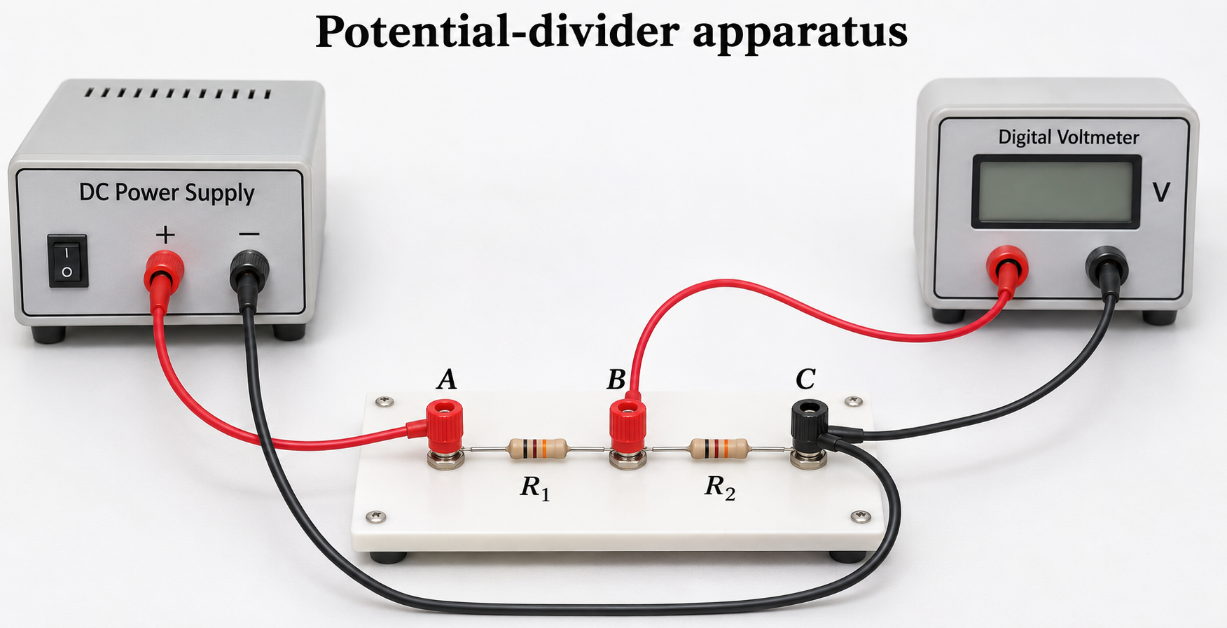

Critical detail
Use two resistors to obtain an output voltage from a supply.

The simple divider formula assumes negligible output loading; this set is not specifically a thermistor or light-sensor circuit.
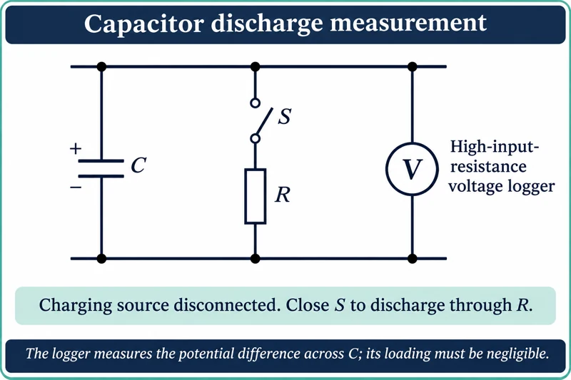 PHYSICS · P32 · 3 VISUALSCapacitor dischargeFollow the voltage across a capacitor as it discharges through a resistor.
Labelled schematic
Follow the voltage across a capacitor as it discharges through a resistor.


Realistic apparatus view
Follow the voltage across a capacitor as it discharges through a resistor.


Critical detail
Follow the voltage across a capacitor as it discharges through a resistor.

The charging source is disconnected; the ideal exponential assumes negligible meter loading and leakage.
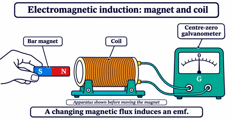 PHYSICS · P33 · 3 VISUALSMagnet and coil inductionMove a magnet relative to a coil and observe the induced electrical response.
Labelled schematic
Move a magnet relative to a coil and observe the induced electrical response.


Realistic apparatus view
Move a magnet relative to a coil and observe the induced electrical response.

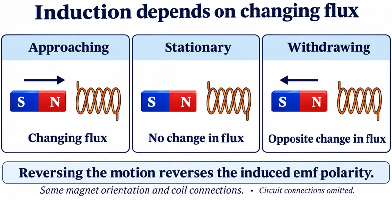
Critical detail
Move a magnet relative to a coil and observe the induced electrical response.

The apparatus starts stationary; the detail compares motion without assigning a universal voltage polarity.
 PHYSICS · P34 · 3 VISUALSTransformer investigationApply low-voltage alternating input to one coil and compare the voltage across another coil on a shared core.
Labelled schematic
Apply low-voltage alternating input to one coil and compare the voltage across another coil on a shared core.


Realistic apparatus view
Apply low-voltage alternating input to one coil and compare the voltage across another coil on a shared core.
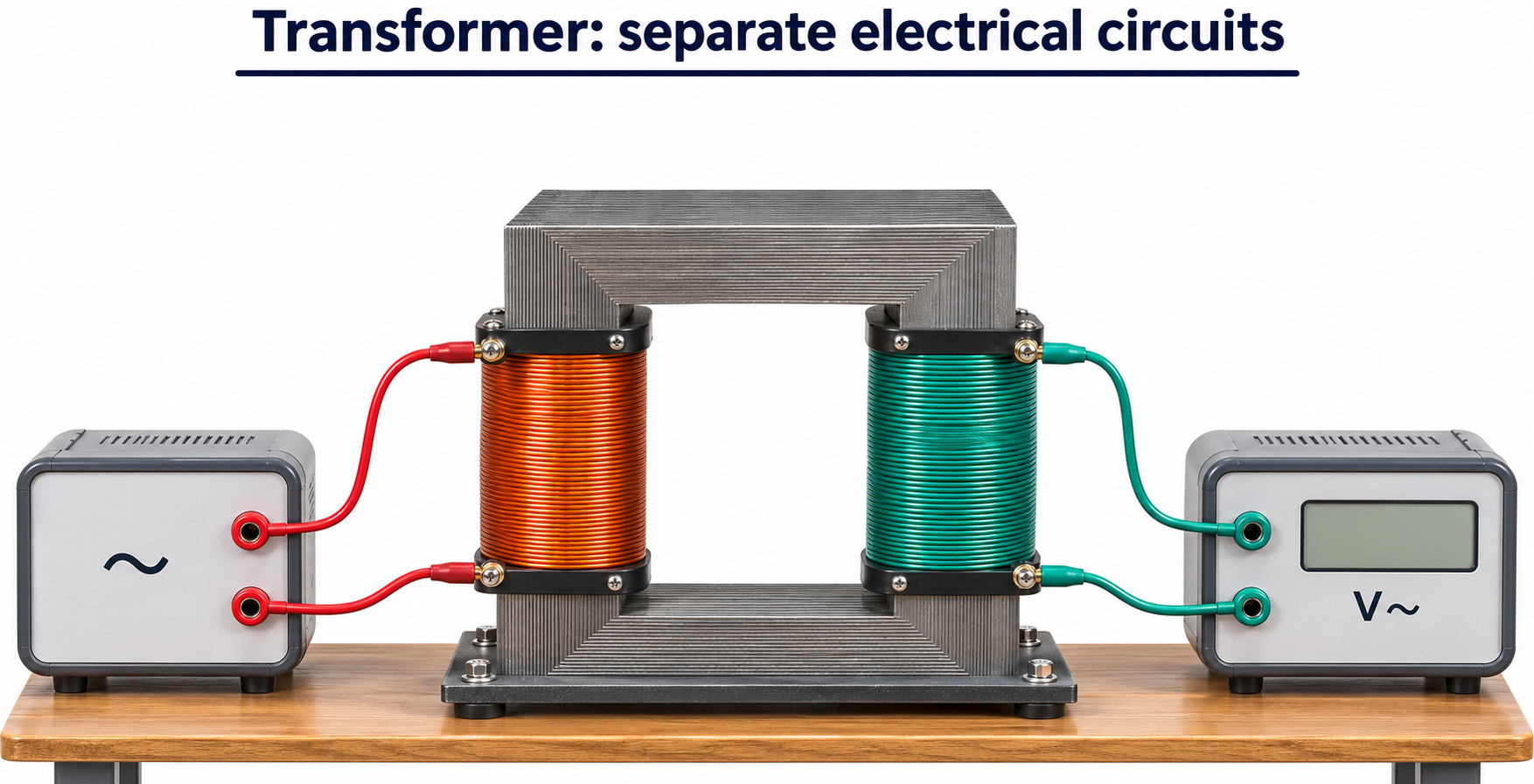

Critical detail
Apply low-voltage alternating input to one coil and compare the voltage across another coil on a shared core.

The turns-ratio relation is idealised and uses corresponding AC voltage measures; real transformers have losses.
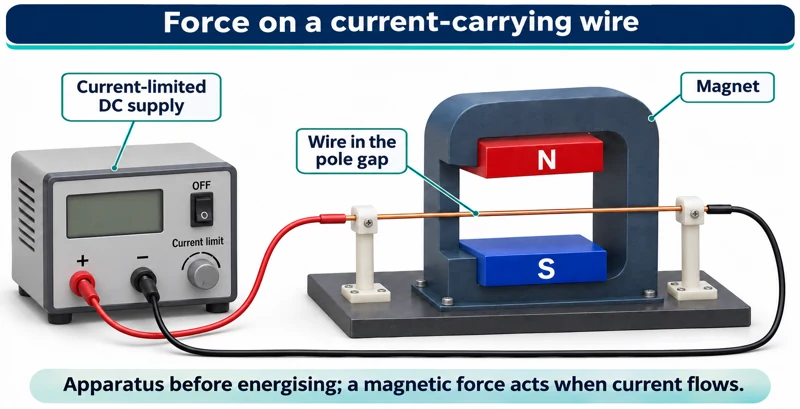 PHYSICS · P35 · 3 VISUALSForce on a current-carrying wirePlace a current-carrying conductor between magnetic poles to investigate the motor effect.
Labelled schematic
Place a current-carrying conductor between magnetic poles to investigate the motor effect.


Realistic apparatus view
Place a current-carrying conductor between magnetic poles to investigate the motor effect.
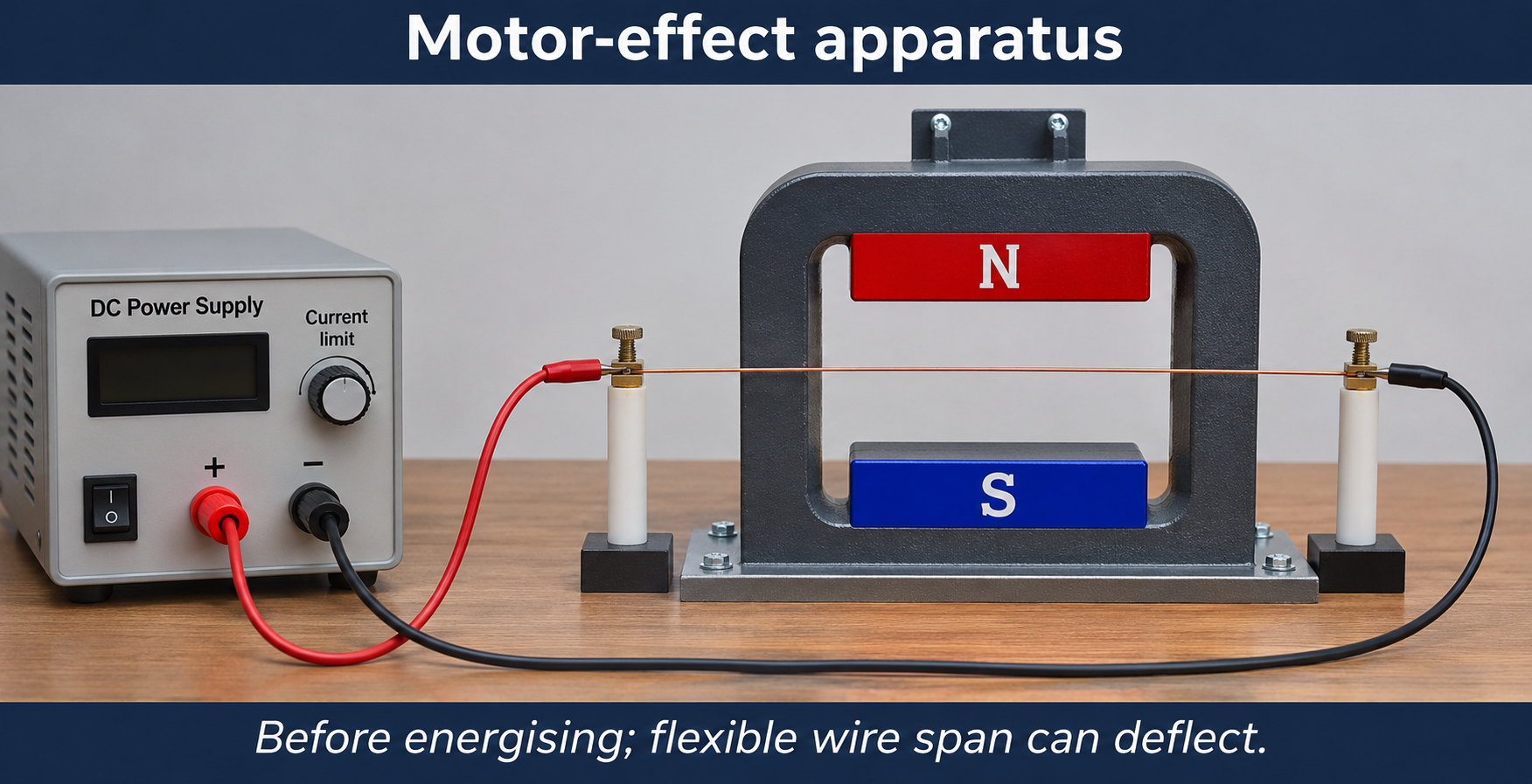
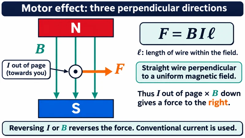
Critical detail
Place a current-carrying conductor between magnetic poles to investigate the motor effect.

The force direction depends on both conventional current and magnetic-field direction; the detail gives one specified orientation.
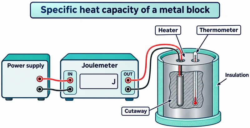 PHYSICS · P36 · 3 VISUALSSpecific heat capacity of a blockMeasure a block's temperature rise after a measured electrical energy input.
Labelled schematic
Measure a block's temperature rise after a measured electrical energy input.


Realistic apparatus view
Measure a block's temperature rise after a measured electrical energy input.
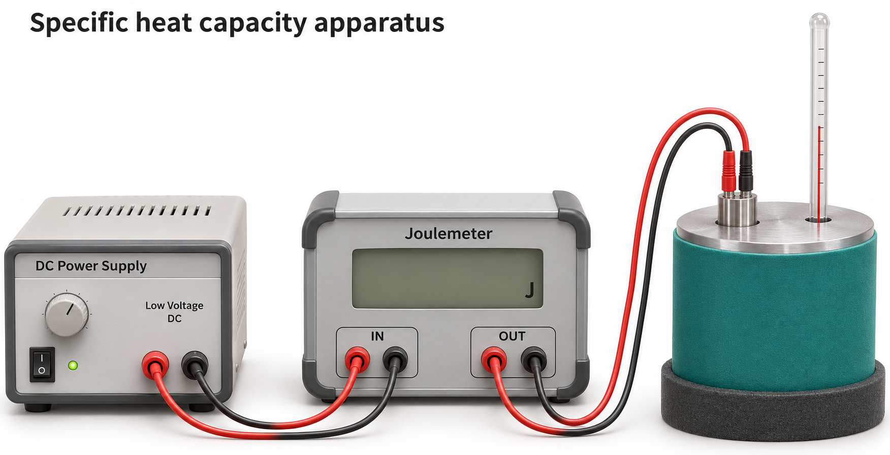

Critical detail
Measure a block's temperature rise after a measured electrical energy input.

The estimate is affected by heat loss and energy absorbed by the heater and other apparatus.
 PHYSICS · P37 · 3 VISUALSLatent heat of fusionCompare meltwater from heated and control ice arrangements to estimate latent heat.
Labelled schematic
Compare meltwater from heated and control ice arrangements to estimate latent heat.


Realistic apparatus view
Compare meltwater from heated and control ice arrangements to estimate latent heat.


Critical detail
Compare meltwater from heated and control ice arrangements to estimate latent heat.
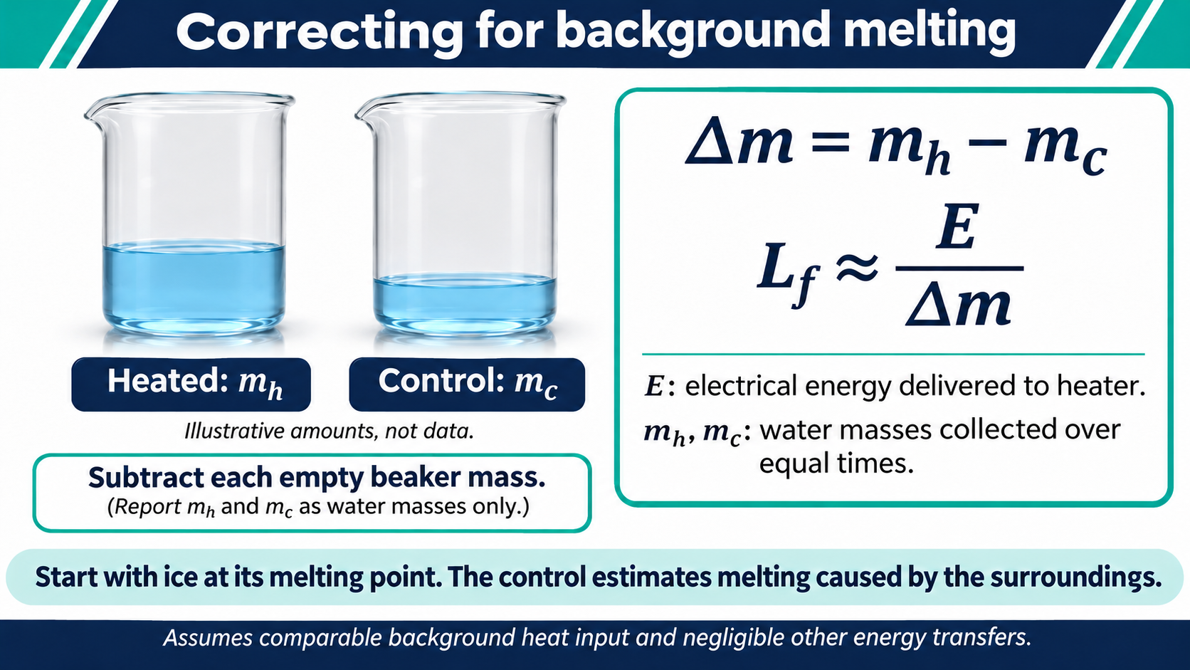
Equal collection times and comparable background melting are required for the control subtraction.
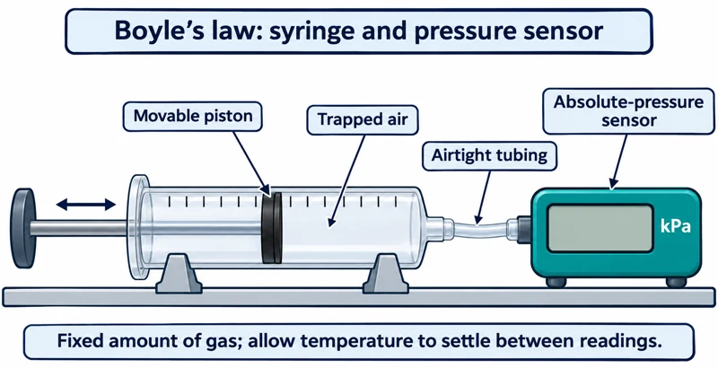 PHYSICS · P38 · 3 VISUALSBoyle's law with a gas syringeMeasure pressure as the volume of a fixed amount of gas is changed.
Labelled schematic
Measure pressure as the volume of a fixed amount of gas is changed.


Realistic apparatus view
Measure pressure as the volume of a fixed amount of gas is changed.


Critical detail
Measure pressure as the volume of a fixed amount of gas is changed.

Use absolute pressure and account for tubing and sensor dead volume while keeping temperature approximately constant.
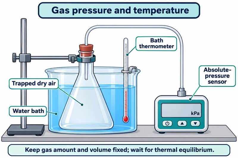 PHYSICS · P39 · 3 VISUALSGas pressure and temperatureMeasure gas pressure in a fixed-volume container as its temperature changes.
Labelled schematic
Measure gas pressure in a fixed-volume container as its temperature changes.


Realistic apparatus view
Measure gas pressure in a fixed-volume container as its temperature changes.

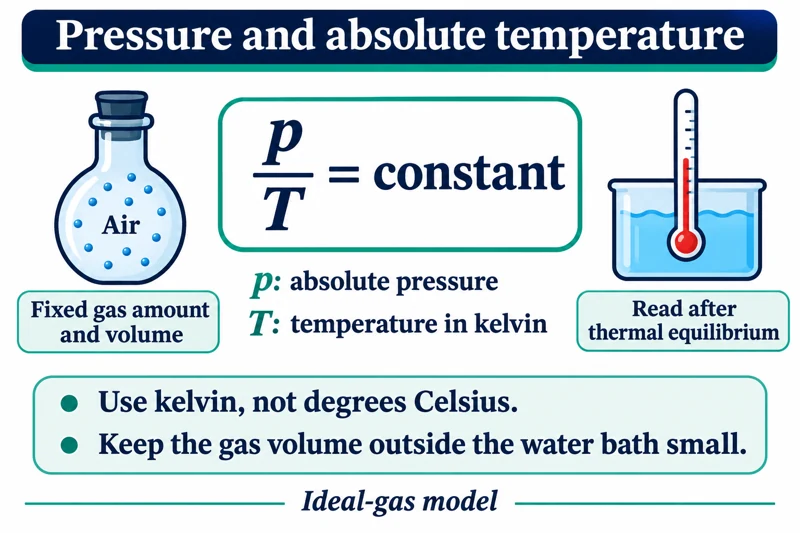
Critical detail
Measure gas pressure in a fixed-volume container as its temperature changes.

Use kelvin and absolute pressure; gas outside the bath may not share the measured temperature.
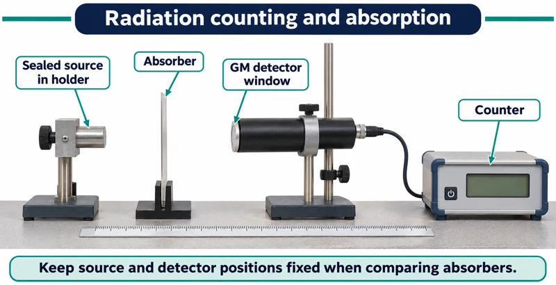 PHYSICS · P40 · 3 VISUALSRadiation counting and absorptionUse a detector, source holder and absorbers to compare measured count rates.
Labelled schematic
Use a detector, source holder and absorbers to compare measured count rates.


Realistic apparatus view
Use a detector, source holder and absorbers to compare measured count rates.
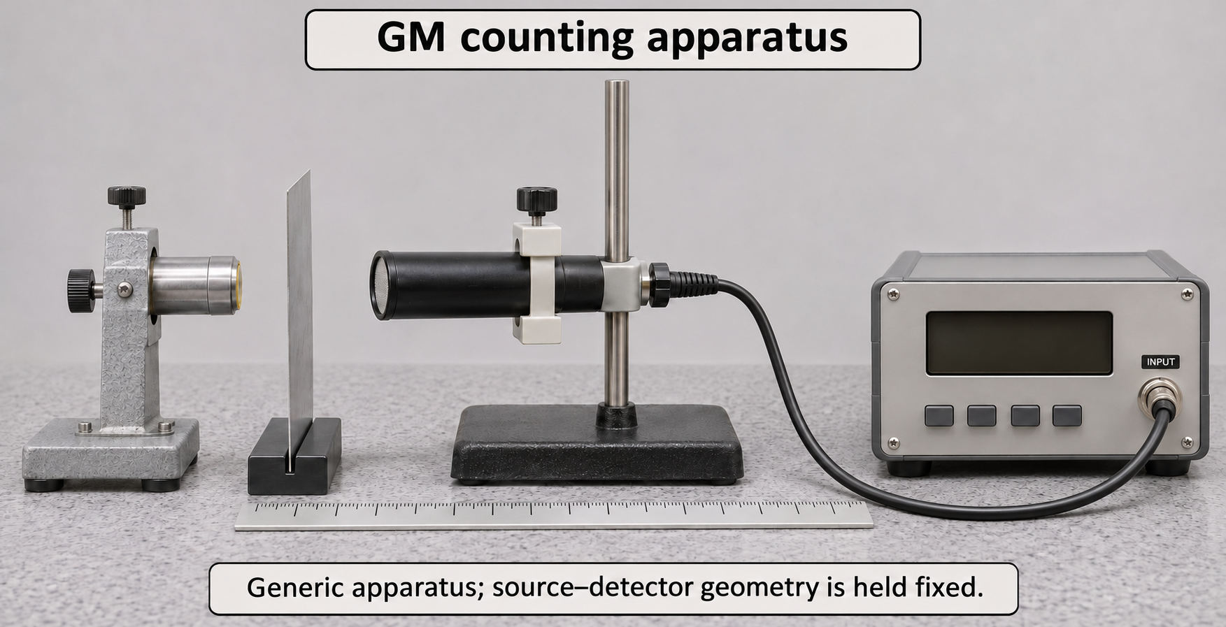

Critical detail
Use a detector, source holder and absorbers to compare measured count rates.

Subtract background count rates using their respective counting times; count rate is not directly a dose measurement.
No matching visuals
Try “cell”, “nucleus” or a different level.
LESS SEARCHING. MORE TEACHING.
From a visual
to an “I get it.”
Choose your detail
Pick a clear overview or a richer view to match what you are explaining.
Look a little closer
Open a large preview before deciding which image belongs in your lesson.
Take it to class
Download the original PNG individually, or download the complete set in one ZIP.